Chapter 10 One-way ANOVA
10.1 Videos
10.1.1 One-Way, Between-Subjects ANOVA
One-Way ANOVA Basics (only first 33 minutes, the rest is on SPSS)
Between-subjects ANOVA and multiple comparisons in R - 11 minutes
10.1.2 Repeated Measures ANOVA
Within-subjects ANOVA basics - 27 min.
This chapter introduces one of the most widely used tools in statistics, known as “the analysis of variance,” which is usually referred to as ANOVA. The basic technique was developed by Sir Ronald Fisher in the early 20th century, and it is to him that we owe the rather unfortunate terminology. The term ANOVA is a little misleading, in two respects. Firstly, although the name of the technique refers to variances, ANOVA is concerned with investigating differences in means. Secondly, there are several different things out there that are all referred to as ANOVAs, some of which have only a very tenuous connection to one another. Later on in the book we’ll encounter a range of different ANOVA methods that apply in quite different situations, but for the purposes of this chapter we’ll only consider the simplest form of ANOVA, in which we have several different groups of observations, and we’re interested in finding out whether those groups differ in terms of some outcome variable of interest. This is the question that is addressed by a one-way ANOVA.
The structure of this chapter is as follows: In Section 10.2 I’ll introduce a fictitious data set that we’ll use as a running example throughout the chapter. After introducing the data, I’ll describe the mechanics of how a one-way ANOVA actually works (Section 10.3) and then focus on how you can run one in R (Section 10.4). These two sections are the core of the chapter. The remainder of the chapter discusses a range of important topics that inevitably arise when running an ANOVA, namely how to calculate effect sizes (Section 10.5), post hoc tests and corrections for multiple comparisons (Section 11.1) and the assumptions that ANOVA relies upon (Section 11.2). We’ll also talk about how to check those assumptions and some of the things you can do if the assumptions are violated (Sections 11.3 to 11.6). At the end of the chapter we’ll talk a little about the relationship between ANOVA and other statistical tools (Section 10.6).
10.2 An illustrative data set
Suppose you’ve become involved in a clinical trial in which you are testing a new antidepressant drug called Joyzepam. In order to construct a fair test of the drug’s effectiveness, the study involves three separate drugs to be administered. One is a placebo, and the other is an existing antidepressant / anti-anxiety drug called Anxifree. A collection of 18 participants with moderate to severe depression are recruited for your initial testing. Because the drugs are sometimes administered in conjunction with psychological therapy, your study includes 9 people undergoing cognitive behavioural therapy (CBT) and 9 who are not. Participants are randomly assigned (doubly blinded, of course) a treatment, such that there are 3 CBT people and 3 no-therapy people assigned to each of the 3 drugs. A psychologist assesses the mood of each person after a 3 month run with each drug: and the overall improvement in each person’s mood is assessed on a scale ranging from \(-5\) to \(+5\).
With that as the study design, let’s now look at what we’ve got in the data file:
load(file.path(projecthome, "data", "clinicaltrial.Rdata")) # load data
str(clin.trial)
## 'data.frame': 18 obs. of 3 variables:
## $ drug : Factor w/ 3 levels "placebo","anxifree",..: 1 1 1 2 2 2 3 3 3 1 ...
## $ therapy : Factor w/ 2 levels "no.therapy","CBT": 1 1 1 1 1 1 1 1 1 2 ...
## $ mood.gain: num 0.5 0.3 0.1 0.6 0.4 0.2 1.4 1.7 1.3 0.6 ...So we have a single data frame called clin.trial, containing three variables; drug, therapy and mood.gain. Next, let’s print the data frame to get a sense of what the data actually look like.
print( clin.trial )## drug therapy mood.gain
## 1 placebo no.therapy 0.5
## 2 placebo no.therapy 0.3
## 3 placebo no.therapy 0.1
## 4 anxifree no.therapy 0.6
## 5 anxifree no.therapy 0.4
## 6 anxifree no.therapy 0.2
## 7 joyzepam no.therapy 1.4
## 8 joyzepam no.therapy 1.7
## 9 joyzepam no.therapy 1.3
## 10 placebo CBT 0.6
## 11 placebo CBT 0.9
## 12 placebo CBT 0.3
## 13 anxifree CBT 1.1
## 14 anxifree CBT 0.8
## 15 anxifree CBT 1.2
## 16 joyzepam CBT 1.8
## 17 joyzepam CBT 1.3
## 18 joyzepam CBT 1.4For the purposes of this chapter, what we’re really interested in is the effect of drug on mood.gain. The first thing to do is calculate some descriptive statistics and draw some graphs. In Chapter 3 we discussed a variety of different functions that can be used for this purpose. For instance, we can use the xtabs() function to see how many people we have in each group:
xtabs( ~drug, clin.trial )## drug
## placebo anxifree joyzepam
## 6 6 6Similarly, we can use the aggregate() function to calculate means and standard deviations for the mood.gain variable broken down by which drug was administered:
aggregate( mood.gain ~ drug, clin.trial, mean )## drug mood.gain
## 1 placebo 0.4500000
## 2 anxifree 0.7166667
## 3 joyzepam 1.4833333aggregate( mood.gain ~ drug, clin.trial, sd )## drug mood.gain
## 1 placebo 0.2810694
## 2 anxifree 0.3920034
## 3 joyzepam 0.2136976Finally, we can use plotmeans() from the gplots package to produce a pretty picture.
library(gplots)
plotmeans(  formula = mood.gain ~ drug,  # plot mood.gain by drug
             data = clin.trial,           # the data frame
             xlab = "Drug Administered",  # x-axis label
             ylab = "Mood Gain",          # y-axis label
             n.label = FALSE              # don't display sample size
 )
The results are shown in Figure 10.1, which plots the average mood gain for all three conditions; error bars show 95% confidence intervals. As the plot makes clear, there is a larger improvement in mood for participants in the Joyzepam group than for either the Anxifree group or the placebo group. The Anxifree group shows a larger mood gain than the control group, but the difference isn’t as large.
The question that we want to answer is: are these difference “real,” or are they just due to chance?
##
## Attaching package: 'gplots'
## The following object is masked from 'package:stats':
##
## lowess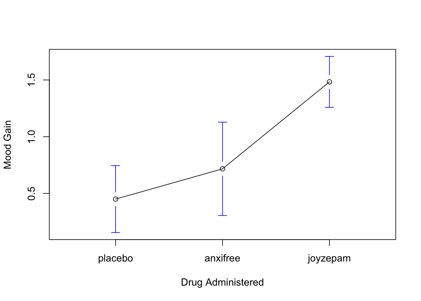
Figure 10.1: Average mood gain as a function of drug administered. Error bars depict 95% confidence intervals associated with each of the group means.
10.3 How ANOVA works
In order to answer the question posed by our clinical trial data, we’re going to run a one-way ANOVA. As usual, I’m going to start by showing you how to do it the hard way, building the statistical tool from the ground up and showing you how you could do it in R if you didn’t have access to any of the cool built-in ANOVA functions. And, as always, I hope you’ll read it carefully, try to do it the long way once or twice to make sure you really understand how ANOVA works, and then – once you’ve grasped the concept – never ever do it this way again.
The experimental design that I described in the previous section strongly suggests that we’re interested in comparing the average mood change for the three different drugs. In that sense, we’re talking about an analysis similar to the \(t\)-test (Chapter 9, but involving more than two groups. If we let \(\mu_P\) denote the population mean for the mood change induced by the placebo, and let \(\mu_A\) and \(\mu_J\) denote the corresponding means for our two drugs, Anxifree and Joyzepam, then the (somewhat pessimistic) null hypothesis that we want to test is that all three population means are identical: that is, neither of the two drugs is any more effective than a placebo. Mathematically, we write this null hypothesis like this: \[ \begin{array}{rcl} H_0 &:& \mbox{it is true that } \mu_P = \mu_A = \mu_J \end{array} \] As a consequence, our alternative hypothesis is that at least one of the three different treatments is different from the others. It’s a little trickier to write this mathematically, because (as we’ll discuss) there are quite a few different ways in which the null hypothesis can be false. So for now we’ll just write the alternative hypothesis like this: \[ \begin{array}{rcl} H_1 &:& \mbox{it is *not* true that } \mu_P = \mu_A = \mu_J \end{array} \] This null hypothesis is a lot trickier to test than any of the ones we’ve seen previously. How shall we do it? A sensible guess would be to “do an ANOVA,” since that’s the title of the chapter, but it’s not particularly clear why an “analysis of variances” will help us learn anything useful about the means. In fact, this is one of the biggest conceptual difficulties that people have when first encountering ANOVA. To see how this works, I find it most helpful to start by talking about variances. In fact, what I’m going to do is start by playing some mathematical games with the formula that describes the variance. That is, we’ll start out by playing around with variances, and it will turn out that this gives us a useful tool for investigating means.
10.3.1 Two formulas for the variance of \(Y\)
Firstly, let’s start by introducing some notation. We’ll use \(G\) to refer to the total number of groups. For our data set, there are three drugs, so there are \(G=3\) groups. Next, we’ll use \(N\) to refer to the total sample size: there are a total of \(N=18\) people in our data set. Similarly, let’s use \(N_k\) to denote the number of people in the \(k\)-th group. In our fake clinical trial, the sample size is \(N_k = 6\) for all three groups.149 Finally, we’ll use \(Y\) to denote the outcome variable: in our case, \(Y\) refers to mood change. Specifically, we’ll use \(Y_{ik}\) to refer to the mood change experienced by the \(i\)-th member of the \(k\)-th group. Similarly, we’ll use \(\bar{Y}\) to be the average mood change, taken across all 18 people in the experiment, and \(\bar{Y}_k\) to refer to the average mood change experienced by the 6 people in group \(k\).
Excellent. Now that we’ve got our notation sorted out, we can start writing down formulas. To start with, let’s recall the formula for the variance that we used in Section 3.4, way back in those kinder days when we were just doing descriptive statistics. The sample variance of \(Y\) is defined as follows: \[ \mbox{Var}(Y) = \frac{1}{N} \sum_{k=1}^G \sum_{i=1}^{N_k} \left(Y_{ik} - \bar{Y} \right)^2 \] This formula looks pretty much identical to the formula for the variance in Section 3.4. The only difference is that this time around I’ve got two summations here: I’m summing over groups (i.e., values for \(k\)) and over the people within the groups (i.e., values for \(i\)). This is purely a cosmetic detail: if I’d instead used the notation \(Y_p\) to refer to the value of the outcome variable for person \(p\) in the sample, then I’d only have a single summation. The only reason that we have a double summation here is that I’ve classified people into groups, and then assigned numbers to people within groups.
A concrete example might be useful here. Let’s consider this table, in which we have a total of \(N=5\) people sorted into \(G=2\) groups. Arbitrarily, let’s say that the “cool” people are group 1, and the “uncool” people are group 2, and it turns out that we have three cool people (\(N_1 = 3\)) and two uncool people (\(N_2 = 2\)).
| name | person (\(p\)) | group | group num (\(k\)) | index in group (\(i\)) | grumpiness (\(Y_{ik}\) or \(Y_p\)) |
|---|---|---|---|---|---|
| Ann | 1 | cool | 1 | 1 | 20 |
| Ben | 2 | cool | 1 | 2 | 55 |
| Cat | 3 | cool | 1 | 3 | 21 |
| Dan | 4 | uncool | 2 | 1 | 91 |
| Egg | 5 | uncool | 2 | 2 | 22 |
Notice that I’ve constructed two different labelling schemes here. We have a “person” variable \(p\), so it would be perfectly sensible to refer to \(Y_p\) as the grumpiness of the \(p\)-th person in the sample. For instance, the table shows that Dan is the four so we’d say \(p = 4\). So, when talking about the grumpiness \(Y\) of this “Dan” person, whoever he might be, we could refer to his grumpiness by saying that \(Y_p = 91\), for person \(p = 4\) that is. However, that’s not the only way we could refer to Dan. As an alternative we could note that Dan belongs to the “uncool” group (\(k = 2\)), and is in fact the first person listed in the uncool group (\(i = 1\)). So it’s equally valid to refer to Dan’s grumpiness by saying that \(Y_{ik} = 91\), where \(k = 2\) and \(i = 1\). In other words, each person \(p\) corresponds to a unique \(ik\) combination, and so the formula that I gave above is actually identical to our original formula for the variance, which would be \[ \mbox{Var}(Y) = \frac{1}{N} \sum_{p=1}^N \left(Y_{p} - \bar{Y} \right)^2 \] In both formulas, all we’re doing is summing over all of the observations in the sample. Most of the time we would just use the simpler \(Y_p\) notation: the equation using \(Y_p\) is clearly the simpler of the two. However, when doing an ANOVA it’s important to keep track of which participants belong in which groups, and we need to use the \(Y_{ik}\) notation to do this.
10.3.2 From variances to sums of squares
Okay, now that we’ve got a good grasp on how the variance is calculated, let’s define something called the total sum of squares, which is denoted SS\(_{tot}\). This is very simple: instead of averaging the squared deviations, which is what we do when calculating the variance, we just add them up. So the formula for the total sum of squares is almost identical to the formula for the variance: \[ \mbox{SS}_{tot} = \sum_{k=1}^G \sum_{i=1}^{N_k} \left(Y_{ik} - \bar{Y} \right)^2 \] When we talk about analysing variances in the context of ANOVA, what we’re really doing is working with the total sums of squares rather than the actual variance. One very nice thing about the total sum of squares is that we can break it up into two different kinds of variation. Firstly, we can talk about the within-group sum of squares, in which we look to see how different each individual person is from their own group mean: \[ \mbox{SS}_w = \sum_{k=1}^G \sum_{i=1}^{N_k} \left( Y_{ik} - \bar{Y}_k \right)^2 \] where \(\bar{Y}_k\) is a group mean. In our example, \(\bar{Y}_k\) would be the average mood change experienced by those people given the \(k\)-th drug. So, instead of comparing individuals to the average of all people in the experiment, we’re only comparing them to those people in the the same group. As a consequence, you’d expect the value of \(\mbox{SS}_w\) to be smaller than the total sum of squares, because it’s completely ignoring any group differences – that is, the fact that the drugs (if they work) will have different effects on people’s moods.
Next, we can define a third notion of variation which captures only the differences between groups. We do this by looking at the differences between the group means \(\bar{Y}_k\) and grand mean \(\bar{Y}\). In order to quantify the extent of this variation, what we do is calculate the between-group sum of squares: \[ \begin{array}{rcl} \mbox{SS}_{b} &=& \sum_{k=1}^G \sum_{i=1}^{N_k} \left( \bar{Y}_k - \bar{Y} \right)^2 \\ &=& \sum_{k=1}^G N_k \left( \bar{Y}_k - \bar{Y} \right)^2 \end{array} \] It’s not too difficult to show that the total variation among people in the experiment \(\mbox{SS}_{tot}\) is actually the sum of the differences between the groups \(\mbox{SS}_b\) and the variation inside the groups \(\mbox{SS}_w\). That is: \[ \mbox{SS}_w + \mbox{SS}_{b} = \mbox{SS}_{tot} \] Yay.
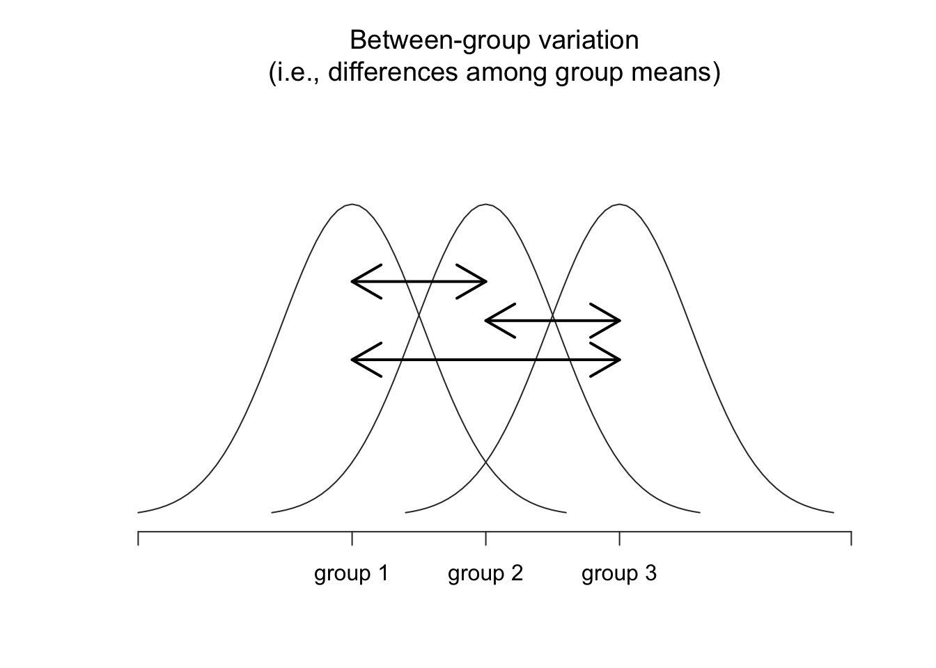
Figure 10.2: Graphical illustration of “between groups” variation
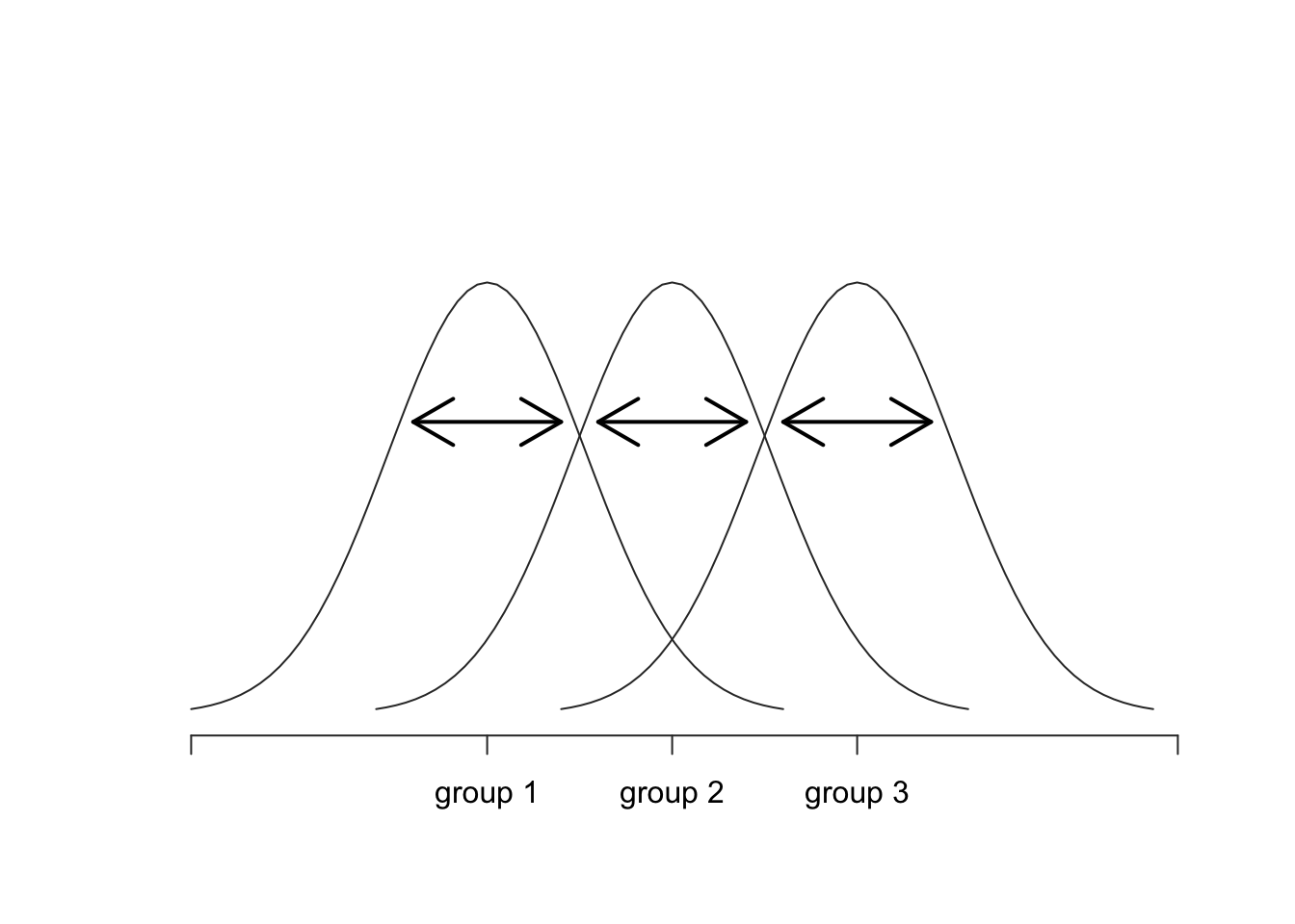
Figure 10.3: Graphical illustration of “within groups” variation
Okay, so what have we found out? We’ve discovered that the total variability associated with the outcome variable (\(\mbox{SS}_{tot}\)) can be mathematically carved up into the sum of “the variation due to the differences in the sample means for the different groups” (\(\mbox{SS}_{b}\)) plus “all the rest of the variation” (\(\mbox{SS}_{w}\)). How does that help me find out whether the groups have different population means? Um. Wait. Hold on a second… now that I think about it, this is exactly what we were looking for. If the null hypothesis is true, then you’d expect all the sample means to be pretty similar to each other, right? And that would imply that you’d expect \(\mbox{SS}_{b}\) to be really small, or at least you’d expect it to be a lot smaller than the “the variation associated with everything else,” \(\mbox{SS}_{w}\). Hm. I detect a hypothesis test coming on…
10.3.3 From sums of squares to the \(F\)-test
As we saw in the last section, the qualitative idea behind ANOVA is to compare the two sums of squares values \(\mbox{SS}_b\) and \(\mbox{SS}_w\) to each other: if the between-group variation is \(\mbox{SS}_b\) is large relative to the within-group variation \(\mbox{SS}_w\) then we have reason to suspect that the population means for the different groups aren’t identical to each other. In order to convert this into a workable hypothesis test, there’s a little bit of “fiddling around” needed. What I’ll do is first show you what we do to calculate our test statistic – which is called an \(F\) ratio – and then try to give you a feel for why we do it this way.
In order to convert our SS values into an \(F\)-ratio, the first thing we need to calculate is the degrees of freedom associated with the SS\(_b\) and SS\(_w\) values. As usual, the degrees of freedom corresponds to the number of unique “data points” that contribute to a particular calculation, minus the number of “constraints” that they need to satisfy. For the within-groups variability, what we’re calculating is the variation of the individual observations (\(N\) data points) around the group means (\(G\) constraints). In contrast, for the between groups variability, we’re interested in the variation of the group means (\(G\) data points) around the grand mean (1 constraint). Therefore, the degrees of freedom here are: \[ \begin{array}{lcl} \mbox{df}_b &=& G-1 \\ \mbox{df}_w &=& N-G \\ \end{array} \] Okay, that seems simple enough. What we do next is convert our summed squares value into a “mean squares” value, which we do by dividing by the degrees of freedom: \[ \begin{array}{lcl} \mbox{MS}_b &=& \displaystyle\frac{\mbox{SS}_b }{ \mbox{df}_b} \\ \mbox{MS}_w &=& \displaystyle\frac{\mbox{SS}_w }{ \mbox{df}_w} \end{array} \] Finally, we calculate the \(F\)-ratio by dividing the between-groups MS by the within-groups MS: \[ F = \frac{\mbox{MS}_b }{ \mbox{MS}_w } \] At a very general level, the intuition behind the \(F\) statistic is straightforward: bigger values of \(F\) means that the between-groups variation is large, relative to the within-groups variation. As a consequence, the larger the value of \(F\), the more evidence we have against the null hypothesis. But how large does \(F\) have to be in order to actually reject \(H_0\)? In order to understand this, you need a slightly deeper understanding of what ANOVA is and what the mean squares values actually are.
The next section discusses that in a bit of detail, but for readers that aren’t interested in the details of what the test is actually measuring, I’ll cut to the chase. In order to complete our hypothesis test, we need to know the sampling distribution for \(F\) if the null hypothesis is true. Not surprisingly, the sampling distribution for the \(F\) statistic under the null hypothesis is an \(F\) distribution. If you recall back to our discussion of the \(F\) distribution in Chapter @ref(probability, the \(F\) distribution has two parameters, corresponding to the two degrees of freedom involved: the first one df\(_1\) is the between groups degrees of freedom df\(_b\), and the second one df\(_2\) is the within groups degrees of freedom df\(_w\).
A summary of all the key quantities involved in a one-way ANOVA, including the formulas showing how they are calculated, is shown in Table 10.1.
| df | sum of squares | mean squares | \(F\) statistic | \(p\) value | |
|---|---|---|---|---|---|
| between groups | \(\mbox{df}_b = G-1\) | SS\(_b = \displaystyle\sum_{k=1}^G N_k (\bar{Y}_k - \bar{Y})^2\) | \(\mbox{MS}_b = \frac{\mbox{SS}_b}{\mbox{df}_b}\) | \(F = \frac{\mbox{MS}_b }{ \mbox{MS}_w }\) | [complicated] |
| within groups | \(\mbox{df}_w = N-G\) | SS\(_w = \sum_{k=1}^G \sum_{i = 1}^{N_k} ( {Y}_{ik} - \bar{Y}_k)^2\) | \(\mbox{MS}_w = \frac{\mbox{SS}_w}{\mbox{df}_w}\) | - | - |
10.3.4 The model for the data and the meaning of \(F\) (advanced)
At a fundamental level, ANOVA is a competition between two different statistical models, \(H_0\) and \(H_1\). When I described the null and alternative hypotheses at the start of the section, I was a little imprecise about what these models actually are. I’ll remedy that now, though you probably won’t like me for doing so. If you recall, our null hypothesis was that all of the group means are identical to one another. If so, then a natural way to think about the outcome variable \(Y_{ik}\) is to describe individual scores in terms of a single population mean \(\mu\), plus the deviation from that population mean. This deviation is usually denoted \(\epsilon_{ik}\) and is traditionally called the error or residual associated with that observation. Be careful though: just like we saw with the word “significant,” the word “error” has a technical meaning in statistics that isn’t quite the same as its everyday English definition. In everyday language, “error” implies a mistake of some kind; in statistics, it doesn’t (or at least, not necessarily). With that in mind, the word “residual” is a better term than the word “error.” In statistics, both words mean “leftover variability”: that is, “stuff” that the model can’t explain. In any case, here’s what the null hypothesis looks like when we write it as a statistical model: \[ Y_{ik} = \mu + \epsilon_{ik} \] where we make the assumption (discussed later) that the residual values \(\epsilon_{ik}\) are normally distributed, with mean 0 and a standard deviation \(\sigma\) that is the same for all groups. To use the notation that we introduced in Chapter ?? we would write this assumption like this: \[ \epsilon_{ik} \sim \mbox{Normal}(0, \sigma^2) \]
What about the alternative hypothesis, \(H_1\)? The only difference between the null hypothesis and the alternative hypothesis is that we allow each group to have a different population mean. So, if we let \(\mu_k\) denote the population mean for the \(k\)-th group in our experiment, then the statistical model corresponding to \(H_1\) is: \[ Y_{ik} = \mu_k + \epsilon_{ik} \] where, once again, we assume that the error terms are normally distributed with mean 0 and standard deviation \(\sigma\). That is, the alternative hypothesis also assumes that \[ \epsilon \sim \mbox{Normal}(0, \sigma^2) \]
Okay, now that we’ve described the statistical models underpinning \(H_0\) and \(H_1\) in more detail, it’s now pretty straightforward to say what the mean square values are measuring, and what this means for the interpretation of \(F\). I won’t bore you with the proof of this, but it turns out that the within-groups mean square, MS\(_w\), can be viewed as an estimator (in the technical sense: Chapter 4.2 of the error variance \(\sigma^2\). The between-groups mean square MS\(_b\) is also an estimator; but what it estimates is the error variance plus a quantity that depends on the true differences among the group means. If we call this quantity \(Q\), then we can see that the \(F\)-statistic is basically150
\[ F = \frac{\hat{Q} + \hat\sigma^2}{\hat\sigma^2} \] where the true value \(Q=0\) if the null hypothesis is true, and \(Q > 0\) if the alternative hypothesis is true (e.g. ch. 10 Hays 1994). Therefore, at a bare minimum the \(F\) value must be larger than 1 to have any chance of rejecting the null hypothesis. Note that this doesn’t mean that it’s impossible to get an \(F\)-value less than 1. What it means is that, if the null hypothesis is true the sampling distribution of the \(F\) ratio has a mean of 1,151 and so we need to see \(F\)-values larger than 1 in order to safely reject the null.
To be a bit more precise about the sampling distribution, notice that if the null hypothesis is true, both MS\(_b\) and MS\(_w\) are estimators of the variance of the residuals \(\epsilon_{ik}\). If those residuals are normally distributed, then you might suspect that the estimate of the variance of \(\epsilon_{ik}\) is chi-square distributed… because (as discussed in Section ?? that’s what a chi-square distribution is: it’s what you get when you square a bunch of normally-distributed things and add them up. And since the \(F\) distribution is (again, by definition) what you get when you take the ratio between two things that are \(\chi^2\) distributed… we have our sampling distribution. Obviously, I’m glossing over a whole lot of stuff when I say this, but in broad terms, this really is where our sampling distribution comes from.
10.3.5 A worked example
The previous discussion was fairly abstract, and a little on the technical side, so I think that at this point it might be useful to see a worked example. For that, let’s go back to the clinical trial data that I introduced at the start of the chapter. The descriptive statistics that we calculated at the beginning tell us our group means: an average mood gain of 0.45 for the placebo, 0.72 for Anxifree, and 1.48 for Joyzepam. With that in mind, let’s party like it’s 1899152 and start doing some pencil and paper calculations. I’ll only do this for the first 5 observations, because it’s not bloody 1899 and I’m very lazy. Let’s start by calculating \(\mbox{SS}_{w}\), the within-group sums of squares. First, let’s draw up a nice table to help us with our calculations…
| group (\(k\)) | outcome (\(Y_{ik}\)) |
|---|---|
| placebo | 0.5 |
| placebo | 0.3 |
| placebo | 0.1 |
| anxifree | 0.6 |
| anxifree | 0.4 |
At this stage, the only thing I’ve included in the table is the raw data itself: that is, the grouping variable (i.e., drug) and outcome variable (i.e. mood.gain) for each person. Note that the outcome variable here corresponds to the \(Y_{ik}\) value in our equation previously. The next step in the calculation is to write down, for each person in the study, the corresponding group mean; that is, \(\bar{Y}_k\). This is slightly repetitive, but not particularly difficult since we already calculated those group means when doing our descriptive statistics:
| group (\(k\)) | outcome (\(Y_{ik}\)) | group mean (\(\bar{Y}_k\)) |
|---|---|---|
| placebo | 0.5 | 0.45 |
| placebo | 0.3 | 0.45 |
| placebo | 0.1 | 0.45 |
| anxifree | 0.6 | 0.72 |
| anxifree | 0.4 | 0.72 |
Now that we’ve written those down, we need to calculate – again for every person – the deviation from the corresponding group mean. That is, we want to subtract \(Y_{ik} - \bar{Y}_k\). After we’ve done that, we need to square everything. When we do that, here’s what we get:
| group (\(k\)) | outcome (\(Y_{ik}\)) | group mean (\(\bar{Y}_k\)) | dev. from group mean (\(Y_{ik} - \bar{Y}_{k}\)) | squared deviation (\((Y_{ik} - \bar{Y}_{k})^2\)) |
|---|---|---|---|---|
| placebo | 0.5 | 0.45 | 0.05 | 0.0025 |
| placebo | 0.3 | 0.45 | -0.15 | 0.0225 |
| placebo | 0.1 | 0.45 | -0.35 | 0.1225 |
| anxifree | 0.6 | 0.72 | -0.12 | 0.0136 |
| anxifree | 0.4 | 0.72 | -0.32 | 0.1003 |
The last step is equally straightforward. In order to calculate the within-group sum of squares, we just add up the squared deviations across all observations: \[ \begin{array}{rcl} \mbox{SS}_w &=& 0.0025 + 0.0225 + 0.1225 + 0.0136 + 0.1003 \\ &=& 0.2614 \end{array} \]
Of course, if we actually wanted to get the right answer, we’d need to do this for all 18 observations in the data set, not just the first five. We could continue with the pencil and paper calculations if we wanted to, but it’s pretty tedious. Alternatively, it’s not too hard to get R to do it. Here’s how:
outcome <- clin.trial$mood.gain
group <- clin.trial$drug
gp.means <- tapply(outcome,group,mean)
gp.means <- gp.means[group]
dev.from.gp.means <- outcome - gp.means
squared.devs <- dev.from.gp.means ^2
It might not be obvious from inspection what these commands are doing: as a general rule, the human brain seems to just shut down when faced with a big block of programming. However, I strongly suggest that – if you’re like me and tend to find that the mere sight of this code makes you want to look away and see if there’s any beer left in the fridge or a game of footy on the telly – you take a moment and look closely at these commands one at a time. Every single one of these commands is something you’ve seen before somewhere else in the book. There’s nothing novel about them (though I’ll have to admit that the tapply() function takes a while to get a handle on), so if you’re not quite sure how these commands work, this might be a good time to try playing around with them yourself, to try to get a sense of what’s happening. On the other hand, if this does seem to make sense, then you won’t be all that surprised at what happens when I wrap these variables in a data frame, and print it out…
Y <- data.frame( group, outcome, gp.means,
                  dev.from.gp.means, squared.devs )
print(Y, digits = 2)
## group outcome gp.means dev.from.gp.means squared.devs
## 1 placebo 0.5 0.45 0.050 0.0025
## 2 placebo 0.3 0.45 -0.150 0.0225
## 3 placebo 0.1 0.45 -0.350 0.1225
## 4 anxifree 0.6 0.72 -0.117 0.0136
## 5 anxifree 0.4 0.72 -0.317 0.1003
## 6 anxifree 0.2 0.72 -0.517 0.2669
## 7 joyzepam 1.4 1.48 -0.083 0.0069
## 8 joyzepam 1.7 1.48 0.217 0.0469
## 9 joyzepam 1.3 1.48 -0.183 0.0336
## 10 placebo 0.6 0.45 0.150 0.0225
## 11 placebo 0.9 0.45 0.450 0.2025
## 12 placebo 0.3 0.45 -0.150 0.0225
## 13 anxifree 1.1 0.72 0.383 0.1469
## 14 anxifree 0.8 0.72 0.083 0.0069
## 15 anxifree 1.2 0.72 0.483 0.2336
## 16 joyzepam 1.8 1.48 0.317 0.1003
## 17 joyzepam 1.3 1.48 -0.183 0.0336
## 18 joyzepam 1.4 1.48 -0.083 0.0069If you compare this output to the contents of the table I’ve been constructing by hand, you can see that R has done exactly the same calculations that I was doing, and much faster too. So, if we want to finish the calculations of the within-group sum of squares in R, we just ask for the sum() of the squared.devs variable:
SSw <- sum( squared.devs )
print( SSw )
## [1] 1.391667Obviously, this isn’t the same as what I calculated, because R used all 18 observations. But if I’d typed sum( squared.devs[1:5] ) instead, it would have given the same answer that I got earlier.
Okay. Now that we’ve calculated the within groups variation, \(\mbox{SS}_w\), it’s time to turn our attention to the between-group sum of squares, \(\mbox{SS}_b\). The calculations for this case are very similar. The main difference is that, instead of calculating the differences between an observation \(Y_{ik}\) and a group mean \(\bar{Y}_k\) for all of the observations, we calculate the differences between the group means \(\bar{Y}_k\) and the grand mean \(\bar{Y}\) (in this case 0.88) for all of the groups…
| group (\(k\)) | group mean (\(\bar{Y}_k\)) | grand mean (\(\bar{Y}\)) | deviation (\(\bar{Y}_{k} - \bar{Y}\)) | squared deviations (\((\bar{Y}_{k} - \bar{Y})^2\)) |
|---|---|---|---|---|
| placebo | 0.45 | 0.88 | -0.43 | 0.18 |
| anxifree | 0.72 | 0.88 | -0.16 | 0.03 |
| joyzepam | 1.48 | 0.88 | 0.60 | 0.36 |
However, for the between group calculations we need to multiply each of these squared deviations by \(N_k\), the number of observations in the group. We do this because every observation in the group (all \(N_k\) of them) is associated with a between group difference. So if there are six people in the placebo group, and the placebo group mean differs from the grand mean by 0.19, then the total between group variation associated with these six people is \(6 \times 0.16 = 1.14\). So we have to extend our little table of calculations…
| group (\(k\)) | squared deviations (\((\bar{Y}_{k} - \bar{Y})^2\)) | sample size (\(N_k\)) | weighted squared dev (\(N_k (\bar{Y}_{k} - \bar{Y})^2\)) |
|---|---|---|---|
| placebo | 0.18 | 6 | 1.11 |
| anxifree | 0.03 | 6 | 0.16 |
| joyzepam | 0.36 | 6 | 2.18 |
And so now our between group sum of squares is obtained by summing these “weighted squared deviations” over all three groups in the study: \[ \begin{array}{rcl} \mbox{SS}_{b} &=& 1.11 + 0.16 + 2.18 \\ &=& 3.45 \end{array} \] As you can see, the between group calculations are a lot shorter, so you probably wouldn’t usually want to bother using R as your calculator. However, if you did decide to do so, here’s one way you could do it:
gp.means <- tapply(outcome,group,mean)
grand.mean <- mean(outcome)
dev.from.grand.mean <- gp.means - grand.mean
squared.devs <- dev.from.grand.mean ^2
gp.sizes <- tapply(outcome,group,length)
wt.squared.devs <- gp.sizes * squared.devs
Again, I won’t actually try to explain this code line by line, but – just like last time – there’s nothing in there that we haven’t seen in several places elsewhere in the book, so I’ll leave it as an exercise for you to make sure you understand it. Once again, we can dump all our variables into a data frame so that we can print it out as a nice table:
Y <- data.frame( gp.means, grand.mean, dev.from.grand.mean,
                  squared.devs, gp.sizes, wt.squared.devs )
print(Y, digits = 2)
## gp.means grand.mean dev.from.grand.mean squared.devs gp.sizes
## placebo 0.45 0.88 -0.43 0.188 6
## anxifree 0.72 0.88 -0.17 0.028 6
## joyzepam 1.48 0.88 0.60 0.360 6
## wt.squared.devs
## placebo 1.13
## anxifree 0.17
## joyzepam 2.16Clearly, these are basically the same numbers that we got before. There are a few tiny differences, but that’s only because the hand-calculated versions have some small errors caused by the fact that I rounded all my numbers to 2 decimal places at each step in the calculations, whereas R only does it at the end (obviously, R s version is more accurate). Anyway, here’s the R command showing the final step:
SSb <- sum( wt.squared.devs )
print( SSb )
## [1] 3.453333which is (ignoring the slight differences due to rounding error) the same answer that I got when doing things by hand.
Now that we’ve calculated our sums of squares values, \(\mbox{SS}_b\) and \(\mbox{SS}_w\), the rest of the ANOVA is pretty painless. The next step is to calculate the degrees of freedom. Since we have \(G = 3\) groups and \(N = 18\) observations in total, our degrees of freedom can be calculated by simple subtraction:
\[
\begin{array}{lclcl}
\mbox{df}_b &=& G - 1 &=& 2 \\
\mbox{df}_w &=& N - G &=& 15
\end{array}
\]
Next, since we’ve now calculated the values for the sums of squares and the degrees of freedom, for both the within-groups variability and the between-groups variability, we can obtain the mean square values by dividing one by the other:
\[
\begin{array}{lclclcl}
\mbox{MS}_b &=& \displaystyle\frac{\mbox{SS}_b }{ \mbox{df}_b } &=& \displaystyle\frac{3.45}{ 2} &=& 1.73
\end{array}
\]
\[
\begin{array}{lclclcl}
\mbox{MS}_w &=& \displaystyle\frac{\mbox{SS}_w }{ \mbox{df}_w } &=& \displaystyle\frac{1.39}{15} &=& 0.09
\end{array}
\]
We’re almost done. The mean square values can be used to calculate the \(F\)-value, which is the test statistic that we’re interested in. We do this by dividing the between-groups MS value by the and within-groups MS value.
\[
F \ = \ \frac{\mbox{MS}_b }{ \mbox{MS}_w } \ = \ \frac{1.73}{0.09} \ = \ 18.6
\]
Woohooo! This is terribly exciting, yes? Now that we have our test statistic, the last step is to find out whether the test itself gives us a significant result. As discussed in Chapter @ref(hypothesistesting, what we really ought to do is choose an \(\alpha\) level (i.e., acceptable Type I error rate) ahead of time, construct our rejection region, etc etc. But in practice it’s just easier to directly calculate the \(p\)-value. Back in the “old days,” what we’d do is open up a statistics textbook or something and flick to the back section which would actually have a huge lookup table… that’s how we’d “compute” our \(p\)-value, because it’s too much effort to do it any other way. However, since we have access to R, I’ll use the pf() function to do it instead. Now, remember that I explained earlier that the \(F\)-test is always one sided? And that we only reject the null hypothesis for very large \(F\)-values? That means we’re only interested in the upper tail of the \(F\)-distribution. The command that you’d use here would be this…
pf( 18.6, df1 = 2, df2 = 15, lower.tail = FALSE)## [1] 8.672727e-05Therefore, our \(p\)-value comes to 0.0000867, or \(8.67 \times 10^{-5}\) in scientific notation. So, unless we’re being extremely conservative about our Type I error rate, we’re pretty much guaranteed to reject the null hypothesis.
At this point, we’re basically done. Having completed our calculations, it’s traditional to organise all these numbers into an ANOVA table like the one in Table@reftab:anovatable. For our clinical trial data, the ANOVA table would look like this:
| df | sum of squares | mean squares | \(F\)-statistic | \(p\)-value | |
|---|---|---|---|---|---|
| between groups | 2 | 3.45 | 1.73 | 18.6 | \(8.67 \times 10^{-5}\) |
| within groups | 15 | 1.39 | 0.09 | - | - |
These days, you’ll probably never have much reason to want to construct one of these tables yourself, but you will find that almost all statistical software (R included) tends to organise the output of an ANOVA into a table like this, so it’s a good idea to get used to reading them. However, although the software will output a full ANOVA table, there’s almost never a good reason to include the whole table in your write up. A pretty standard way of reporting this result would be to write something like this:
One-way ANOVA showed a significant effect of drug on mood gain (\(F(2,15) = 18.6, p<.001\)).
Sigh. So much work for one short sentence.
10.4 Running an ANOVA in R
I’m pretty sure I know what you’re thinking after reading the last section, especially if you followed my advice and tried typing all the commands in yourself…. doing the ANOVA calculations yourself sucks. There’s quite a lot of calculations that we needed to do along the way, and it would be tedious to have to do this over and over again every time you wanted to do an ANOVA. One possible solution to the problem would be to take all these calculations and turn them into some R functions yourself. You’d still have to do a lot of typing, but at least you’d only have to do it the one time: once you’ve created the functions, you can reuse them over and over again. However, writing your own functions is a lot of work, so this is kind of a last resort. Besides, it’s much better if someone else does all the work for you…
10.4.1 Using the aov() function to specify your ANOVA
To make life easier for you, R provides a function called aov(), which – obviously – is an acronym of “Analysis Of Variance.”153 If you type ?aov and have a look at the help documentation, you’ll see that there are several arguments to the aov() function, but the only two that we’re interested in are formula and data. As we’ve seen in a few places previously, the formula argument is what you use to specify the outcome variable and the grouping variable, and the data argument is what you use to specify the data frame that stores these variables. In other words, to do the same ANOVA that I laboriously calculated in the previous section, I’d use a command like this:
aov( formula = mood.gain ~ drug, data = clin.trial ) Actually, that’s not quite the whole story, as you’ll see as soon as you look at the output from this command, which I’ve hidden for the moment in order to avoid confusing you. Before we go into specifics, I should point out that either of these commands will do the same thing:
aov( clin.trial$mood.gain ~ clin.trial$drug )
aov( mood.gain ~ drug, clin.trial )
In the first command, I didn’t specify a data set, and instead relied on the $ operator to tell R how to find the variables. In the second command, I dropped the argument names, which is okay in this case because formula is the first argument to the aov() function, and data is the second one. Regardless of how I specify the ANOVA, I can assign the output of the aov() function to a variable, like this for example:
my.anova <- aov( mood.gain ~ drug, clin.trial ) This is almost always a good thing to do, because there’s lots of useful things that we can do with the my.anova variable. So let’s assume that it’s this last command that I used to specify the ANOVA that I’m trying to run, and as a consequence I have this my.anova variable sitting in my workspace, waiting for me to do something with it…
10.4.2 Understanding what the aov() function produces
Now that we’ve seen how to use the aov() function to create my.anova we’d better have a look at what this variable actually is. The first thing to do is to check to see what class of variable we’ve created, since it’s kind of interesting in this case. When we do that…
class( my.anova )## [1] "aov" "lm"… we discover that my.anova actually has two classes! The first class tells us that it’s an aov (analysis of variance) object, but the second tells us that it’s also an lm (linear model) object. Later on, we’ll see that this reflects a pretty deep statistical relationship between ANOVA and regression (Chapter 8 and it means that any function that exists in R for dealing with regressions can also be applied to aov objects, which is neat; but I’m getting ahead of myself. For now, I want to note that what we’ve created is an aov object, and to also make the point that aov objects are actually rather complicated beasts. I won’t be trying to explain everything about them, since it’s way beyond the scope of an introductory statistics subject, but to give you a tiny hint of some of the stuff that R stores inside an aov object, let’s ask it to print out the names() of all the stored quantities…
names( my.anova )## [1] "coefficients" "residuals" "effects" "rank"
## [5] "fitted.values" "assign" "qr" "df.residual"
## [9] "contrasts" "xlevels" "call" "terms"
## [13] "model"As we go through the rest of the book, I hope that a few of these will become a little more obvious to you, but right now that’s going to look pretty damned opaque. That’s okay. You don’t need to know any of the details about it right now, and most of it you don’t need at all… what you do need to understand is that the aov() function does a lot of calculations for you, not just the basic ones that I outlined in the previous sections. What this means is that it’s generally a good idea to create a variable like my.anova that stores the output of the aov() function… because later on, you can use my.anova as an input to lots of other functions: those other functions can pull out bits and pieces from the aov object, and calculate various other things that you might need.
Right then. The simplest thing you can do with an aov object is to print() it out. When we do that, it shows us a few of the key quantities of interest:
print( my.anova )## Call:
## aov(formula = mood.gain ~ drug, data = clin.trial)
##
## Terms:
## drug Residuals
## Sum of Squares 3.453333 1.391667
## Deg. of Freedom 2 15
##
## Residual standard error: 0.3045944
## Estimated effects may be unbalancedSpecificially, it prints out a reminder of the command that you used when you called aov() in the first place, shows you the sums of squares values, the degrees of freedom, and a couple of other quantities that we’re not really interested in right now. Notice, however, that R doesn’t use the names “between-group” and “within-group.” Instead, it tries to assign more meaningful names: in our particular example, the between groups variance corresponds to the effect that the drug has on the outcome variable; and the within groups variance is corresponds to the “leftover” variability, so it calls that the residuals. If we compare these numbers to the numbers that I calculated by hand in Section 10.3.5, you can see that they’re identical… the between groups sums of squares is \(\mbox{SS}_b = 3.45\), the within groups sums of squares is \(\mbox{SS}_w = 1.39\), and the degrees of freedom are 2 and 15 repectively.
10.4.3 Running the hypothesis tests for the ANOVA
Okay, so we’ve verified that my.anova seems to be storing a bunch of the numbers that we’re looking for, but the print() function didn’t quite give us the output that we really wanted. Where’s the \(F\)-value? The \(p\)-value? These are the most important numbers in our hypothesis test, but the print() function doesn’t provide them. To get those numbers, we need to use a different function. Instead of asking R to print() out the aov object, we should have asked for a summary() of it.154 When we do that…
summary( my.anova )## Df Sum Sq Mean Sq F value Pr(>F)
## drug 2 3.453 1.7267 18.61 8.65e-05 ***
## Residuals 15 1.392 0.0928
## ---
## Signif. codes: 0 '***' 0.001 '**' 0.01 '*' 0.05 '.' 0.1 ' ' 1… we get all of the key numbers that we calculated earlier. We get the sums of squares, the degrees of freedom, the mean squares, the \(F\)-statistic, and the \(p\)-value itself. These are all identical to the numbers that we calculated ourselves when doing it the long and tedious way, and it’s even organised into the same kind of ANOVA table that I showed in Table 10.1, and then filled out by hand in Section 10.3.5. The only things that are even slightly different is that some of the row and column names are a bit different.
10.5 Effect size
There’s a few different ways you could measure the effect size in an ANOVA, but the most commonly used measures are \(\eta^2\) (eta squared) and partial \(\eta^2\). For a one way analysis of variance they’re identical to each other, so for the moment I’ll just explain \(\eta^2\). The definition of \(\eta^2\) is actually really simple:
\[
\eta^2 = \frac{\mbox{SS}_b}{\mbox{SS}_{tot}}
\]
That’s all it is. So when I look at the ANOVA table above, I see that \(\mbox{SS}_b = 3.45\) and \(\mbox{SS}_{tot} = 3.45 + 1.39 = 4.84\). Thus we get an \(\eta^2\) value of
\[
\eta^2 = \frac{3.45}{4.84} = 0.71
\]
The interpretation of \(\eta^2\) is equally straightforward: it refers to the proportion of the variability in the outcome variable (mood.gain) that can be explained in terms of the predictor (drug). A value of \(\eta^2 = 0\) means that there is no relationship at all between the two, whereas a value of \(\eta^2 = 1\) means that the relationship is perfect. Better yet, the \(\eta^2\) value is very closely related to a squared correlation (i.e., \(r^2\)). So, if you’re trying to figure out whether a particular value of \(\eta^2\) is big or small, it’s sometimes useful to remember that
\[
\eta= \sqrt{\frac{\mbox{SS}_b}{\mbox{SS}_{tot}}}
\]
can be interpreted as if it referred to the magnitude of a Pearson correlation. So in our drugs example, the \(\eta^2\) value of .71 corresponds to an \(\eta\) value of \(\sqrt{.71} = .84\). If we think about this as being equivalent to a correlation of about .84, we’d conclude that the relationship between drug and mood.gain is strong.
The core packages in R don’t include any functions for calculating \(\eta^2\). However, it’s pretty straightforward to calculate it directly from the numbers in the ANOVA table. In fact, since I’ve already got the SSw and SSb variables lying around from my earlier calculations, I can do this:
SStot <- SSb + SSw          # total sums of squares
eta.squared <- SSb / SStot  # eta-squared value
print( eta.squared )
## [1] 0.7127623However, since it can be tedious to do this the long way (especially when we start running more complicated ANOVAs, such as those in Chapter ?? I’ve included an etaSquared() function in the lsr package which will do it for you. For now, the only argument you need to care about is x, which should be the aov object corresponding to your ANOVA. When we do this, what we get as output is this:
etaSquared( x = my.anova )## eta.sq eta.sq.part
## drug 0.7127623 0.7127623The output here shows two different numbers. The first one corresponds to the \(\eta^2\) statistic, precisely as described above. The second one refers to “partial \(\eta^2\),” which is a somewhat different measure of effect size that I’ll describe later. For the simple ANOVA that we’ve just run, they’re the same number. But this won’t always be true once we start running more complicated ANOVAs.155
10.6 On the relationship between ANOVA and the Student \(t\) test
There’s one last thing I want to point out before finishing. It’s something that a lot of people find kind of surprising, but it’s worth knowing about: an ANOVA with two groups is identical to the Student \(t\)-test. No, really. It’s not just that they are similar, but they are actually equivalent in every meaningful way. I won’t try to prove that this is always true, but I will show you a single concrete demonstration. Suppose that, instead of running an ANOVA on our mood.gain ~ drug model, let’s instead do it using therapy as the predictor. If we run this ANOVA, here’s what we get:
summary( aov( mood.gain ~ therapy, data = clin.trial ))## Df Sum Sq Mean Sq F value Pr(>F)
## therapy 1 0.467 0.4672 1.708 0.21
## Residuals 16 4.378 0.2736Overall, it looks like there’s no significant effect here at all but, as we’ll see in Chapter @ref(anova2 this is actually a misleading answer! In any case, it’s irrelevant to our current goals: our interest here is in the \(F\)-statistic, which is \(F(1,16) = 1.71\), and the \(p\)-value, which is .21. Since we only have two groups, I didn’t actually need to resort to an ANOVA, I could have just decided to run a Student \(t\)-test. So let’s see what happens when I do that:
t.test( mood.gain ~ therapy, data = clin.trial, var.equal = TRUE )##
## Two Sample t-test
##
## data: mood.gain by therapy
## t = -1.3068, df = 16, p-value = 0.2098
## alternative hypothesis: true difference in means is not equal to 0
## 95 percent confidence interval:
## -0.8449518 0.2005073
## sample estimates:
## mean in group no.therapy mean in group CBT
## 0.7222222 1.0444444Curiously, the \(p\)-values are identical: once again we obtain a value of \(p = .21\). But what about the test statistic? Having run a \(t\)-test instead of an ANOVA, we get a somewhat different answer, namely \(t(16) = -1.3068\). However, there is a fairly straightforward relationship here. If we square the \(t\)-statistic
1.3068 ^ 2## [1] 1.707726we get the \(F\)-statistic from before.
10.7 Summary
In terms of what we have discussed, the key topics were:
- The basic logic behind how ANOVA works (Section 10.3) and how to run one in R (Section 10.4).
- How to compute an effect size for an ANOVA (Section 10.5)
As with all of the chapters in this book, there are quite a few different sources that I’ve relied upon, but the one stand-out text that I’ve been most heavily influenced by is Sahai and Ageel (2000). It’s not a good book for beginners, but it’s an excellent book for more advanced readers who are interested in understanding the mathematics behind ANOVA.
References
When all groups have the same number of observations, the experimental design is said to be “balanced.” Balance isn’t such a big deal for one-way ANOVA, which is the topic of this chapter. It becomes more important when you start doing more complicated ANOVAs.↩︎
In a later versions I’m intending to expand on this. But because I’m writing in a rush, and am already over my deadlines, I’ll just briefly note that if you read ahead to Chapter ?? and look at how the “treatment effect” at level \(k\) of a factor is defined in terms of the \(\alpha_k\) values (see Section 12.4), it turns out that \(Q\) refers to a weighted mean of the squared treatment effects, \(Q=(\sum_{k=1}^G N_k\alpha_k^2)/(G-1)\).↩︎
Or, if we want to be sticklers for accuracy, \(1 + \frac{2}{df_2 - 2}\).↩︎
Or, to be precise, party like “it’s 1899 and we’ve got no friends and nothing better to do with our time than do some calculations that wouldn’t have made any sense in 1899 because ANOVA didn’t exist until about the 1920s.”↩︎
Actually, it also provides a function called
anova(), but that works a bit differently, so let’s just ignore it for now.↩︎It’s worth noting that you can get the same result by using the command
anova( my.anova ).↩︎A potentially important footnote – I wrote the
etaSquared()function for thelsrpackage as a teaching exercise, but like all the other functions in thelsrpackage it hasn’t been exhaustively tested. As of this writing –lsrpackage version 0.5 – there is at least one known bug in the code. In some cases at least, it doesn’t work (and can give very silly answers) when you set theweightson the observations to something other than uniform. That doesn’t matter at all for this book, since those kinds of analyses are well beyond the scope, but I haven’t had a chance to revisit the package in a long time; it would probably be wise to be very cautious with the use of this function in any context other than very simple introductory analyses. Thanks to Emil Kirkegaard for finding the bug! (Oh, and while I’m here, there’s an interesting blog post by Daniel Lakens suggesting that eta-squared itself is perhaps not the best measure of effect size in real world data analysis: http://daniellakens.blogspot.com.au/2015/06/why-you-should-use-omega-squared.html↩︎