Chapter 2 Getting started with R
2.1 Videos
2.2 Introduction
Robots are nice to work with.
–Roger Zelazny5
In this chapter I’ll discuss how to get started in R. I’ll briefly talk about how to download and install R, but most of the chapter will be focused on getting you started typing R commands. Our goal in this chapter is not to learn any statistical concepts: we’re just trying to learn the basics of how R works and get comfortable interacting with the system. To do this, we’ll spend a bit of time using R as a simple calculator, since that’s the easiest thing to do with R. In doing so, you’ll get a bit of a feel for what it’s like to work in R. From there I’ll introduce some very basic programming ideas: in particular, I’ll talk about the idea of defining variables to store information, and a few things that you can do with these variables.
However, before going into any of the specifics, it’s worth talking a little about why you might want to use R at all. Given that you’re reading this, you’ve probably got your own reasons. However, if those reasons are “because that’s what my stats class uses,” it might be worth explaining a little why your lecturer has chosen to use R for the class. Of course, I don’t really know why other people choose R, so I’m really talking about why I use it.
- It’s sort of obvious, but worth saying anyway: doing your statistics on a computer is faster, easier and more powerful than doing statistics by hand. Computers excel at mindless repetitive tasks, and a lot of statistical calculations are both mindless and repetitive. For most people, the only reason to ever do statistical calculations with pencil and paper is for learning purposes. In my class I do occasionally suggest doing some calculations that way, but the only real value to it is pedagogical. It does help you to get a “feel” for statistics to do some calculations yourself, so it’s worth doing it once. But only once!
- Doing statistics in a spreadsheet (e.g., Microsoft Excel) is generally a bad idea in the long run. Although many people are likely feel more familiar with them, spreadsheets are very limited in terms of what analyses they allow you do. If you get into the habit of trying to do your real life data analysis using spreadsheets, then you’ve dug yourself into a very deep hole.
- Avoiding proprietary software is a very good idea. There are a lot of commercial packages out there that you can buy, some of which I like and some of which I don’t. They’re usually very glossy in their appearance, and generally very powerful (much more powerful than spreadsheets). However, they’re also very expensive: usually, the company sells “student versions” (limited versions of the real thing) very cheaply; they sell full powered “educational versions” at a price that makes me wince; and they sell commercial licences with a staggeringly high price tag. The business model here is to suck you in during your student days, and then leave you dependent on their tools when you go out into the real world. It’s hard to blame them for trying, but personally I’m not in favour of shelling out thousands of dollars if I can avoid it. And you can avoid it: if you make use of packages like R that are open source and free, you never get trapped having to pay exorbitant licensing fees.
- Something that you might not appreciate now, but will love later on if you do anything involving data analysis, is the fact that R is highly extensible. When you download and install R, you get all the basic “packages,” and those are very powerful on their own. However, because R is so open and so widely used, it’s become something of a standard tool in statistics, and so lots of people write their own packages that extend the system. And these are freely available too. One of the consequences of this, I’ve noticed, is that if you open up an advanced textbook (a recent one, that is) rather than introductory textbooks, is that a lot of them use R. In other words, if you learn how to do your basic statistics in R, then you’re a lot closer to being able to use the state of the art methods than you would be if you’d started out with a “simpler” system: so if you want to become a genuine expert in psychological data analysis, learning R is a very good use of your time.
- Related to the previous point: R is a real programming language. As you get better at using R for data analysis, you’re also learning to program. To some people this might seem like a bad thing, but in truth, programming is a core research skill across a lot of the social and behavioural sciences. Think about how many surveys and experiments are done online, or presented on computers. Think about all those online social environments which you might be interested in studying; and maybe collecting data from in an automated fashion. Think about artificial intelligence systems, computer vision and speech recognition. If any of these are things that you think you might want to be involved in – as someone “doing research in psychology,” that is – you’ll need to know a bit of programming. And if you don’t already know how to program, then learning how to do statistics using R is a nice way to start.
Those are the main reasons I use R. It’s not without its flaws: it’s not easy to learn, and it has a few very annoying quirks to it that we’re all pretty much stuck with, but on the whole I think the strengths outweigh the weakness; more so than any other option I’ve encountered so far.
2.3 Installing R
Okay, enough with the sales pitch. Let’s get started. Just as with any piece of software, R needs to be installed on a “computer,” which is a magical box that does cool things and delivers free ponies. Or something along those lines: I may be confusing computers with the iPad marketing campaigns. Anyway, R is freely distributed online, and you can download it from the R homepage, which is:
At the top of the page – under the heading “Download and Install R” – you’ll see separate links for Windows users, Mac users, and Linux users. If you follow the relevant link, you’ll see that the online instructions are pretty self-explanatory, but I’ll walk you through the installation anyway. As of this writing, the current version of R is 3.0.2 (``Frisbee Sailing"), but they usually issue updates every six months, so you’ll probably have a newer version.6
2.3.1 Installing R on a Windows computer
The CRAN homepage changes from time to time, and it’s not particularly pretty, or all that well-designed quite frankly. But it’s not difficult to find what you’re after. In general you’ll find a link at the top of the page with the text “Download R for Windows.” If you click on that, it will take you to a page that offers you a few options. Again, at the very top of the page you’ll be told to click on a link that says to click here if you’re installing R for the first time. That’s probably what you want. This will take you to a page that has a prominent link at the top called “Download R 3.0.2 for Windows.” That’s the one you want. Click on that and your browser should start downloading a file called R-3.0.2-win.exe, or whatever the equivalent version number is by the time you read this. The file for version 3.0.2 is about 54MB in size, so it may take some time depending on how fast your internet connection is. Once you’ve downloaded the file, double click to install it. As with any software you download online, Windows will ask you some questions about whether you trust the file and so on. After you click through those, it’ll ask you where you want to install it, and what components you want to install. The default values should be fine for most people, so again, just click through. Once all that is done, you should have R installed on your system. You can access it from the Start menu, or from the desktop if you asked it to add a shortcut there. You can now open up R in the usual way if you want to, but what I’m going to suggest is that instead of doing that you should now install RStudio (see Section 2.3.4 for instructions).
2.3.2 Installing R on a Mac
When you click on the Mac OS X link, you should find yourself on a page with the title “R for Mac OS X.” The vast majority of Mac users will have a fairly recent version of the operating system: as long as you’re running Mac OS X 10.6 (Snow Leopard) or higher, then you’ll be fine.7 There’s a fairly prominent link on the page called “R-3.0.2.pkg,” which is the one you want. Click on that link and you’ll start downloading the installer file, which is (not surprisingly) called R-3.0.2.pkg. It’s about 61MB in size, so the download can take a while on slower internet connections.
Once you’ve downloaded R-3.0.2.pkg, all you need to do is open it by double clicking on the package file. The installation should go smoothly from there: just follow all the instructions just like you usually do when you install something. Once it’s finished, you’ll find a file called R.app in the Applications folder. You can now open up R in the usual way8 if you want to, but what I’m going to suggest is that instead of doing that you should now install RStudio (see Section 2.3.4 for instructions).
2.3.3 Installing R on a Linux computer
If you’re successfully managing to run a Linux box, regardless of what distribution, then you should find the instructions on the website easy enough. You can compile R from source yourself if you want, or install it through your package management system, which will probably have R in it.
Alternatively, the CRAN site has precompiled binaries for Debian, Red Hat, Suse and Ubuntu and has separate instructions for each. Once you’ve got R installed, you can run it from the command line just by typing R. However, if you’re feeling envious of Windows and Mac users for their fancy GUIs, you can download RStudio too (see Section 2.3.4 for instructions).
2.3.4 Downloading and installing RStudio
Okay, so regardless of what operating system you’re using, the last thing that I told you to do is to download RStudio. To understand why I’ve suggested this, you need to understand a little bit more about R itself. The term R doesn’t really refer to a specific application on your computer. Rather, it refers to the underlying statistical language. You can use this language through lots of different applications. When you install R initially, it comes with one application that lets you do this: it’s the R.exe application on a Windows machine, and the R.app application on a Mac. But that’s not the only way to do it. There are lots of different applications that you can use that will let you interact with R. One of those is called RStudio, and it’s the one I’m going to suggest that you use. RStudio provides a clean, professional interface to R that I find much nicer to work with than either the Windows or Mac defaults. Like R itself, RStudio is free software: you can find all the details on their webpage. In the meantime, you can download it here:
When you visit the RStudio website, you’ll probably be struck by how much cleaner and simpler it is than the CRAN website,9 and how obvious it is what you need to do: click the big green button that says “Download.”
When you click on the download button on the homepage it will ask you to choose whether you want the desktop version or the server version. You want the desktop version. After choosing the desktop version it will take you to a page http://www.RStudio.org/download/desktop) that shows several possible downloads: there’s a different one for each operating system. However, the nice people at RStudio have designed the webpage so that it automatically recommends the download that is most appropriate for your computer. Click on the appropriate link, and the RStudio installer file will start downloading.
Once it’s finished downloading, open the installer file in the usual way to install RStudio. After it’s finished installing, you can start R by opening RStudio. You don’t need to open R.app or R.exe in order to access R. RStudio will take care of that for you. To illustrate what RStudio looks like, Figure 2.1 shows a screenshot of an R session in progress. In this screenshot, you can see that it’s running on a Mac, but it looks almost identical no matter what operating system you have. The Windows version looks more like a Windows application (e.g., the menus are attached to the application window and the colour scheme is slightly different), but it’s more or less identical. There are a few minor differences in where things are located in the menus (I’ll point them out as we go along) and in the shortcut keys, because RStudio is trying to “feel” like a proper Mac application or a proper Windows application, and this means that it has to change its behaviour a little bit depending on what computer it’s running on. Even so, these differences are very small: I started out using the Mac version of RStudio and then started using the Windows version as well in order to write these notes.
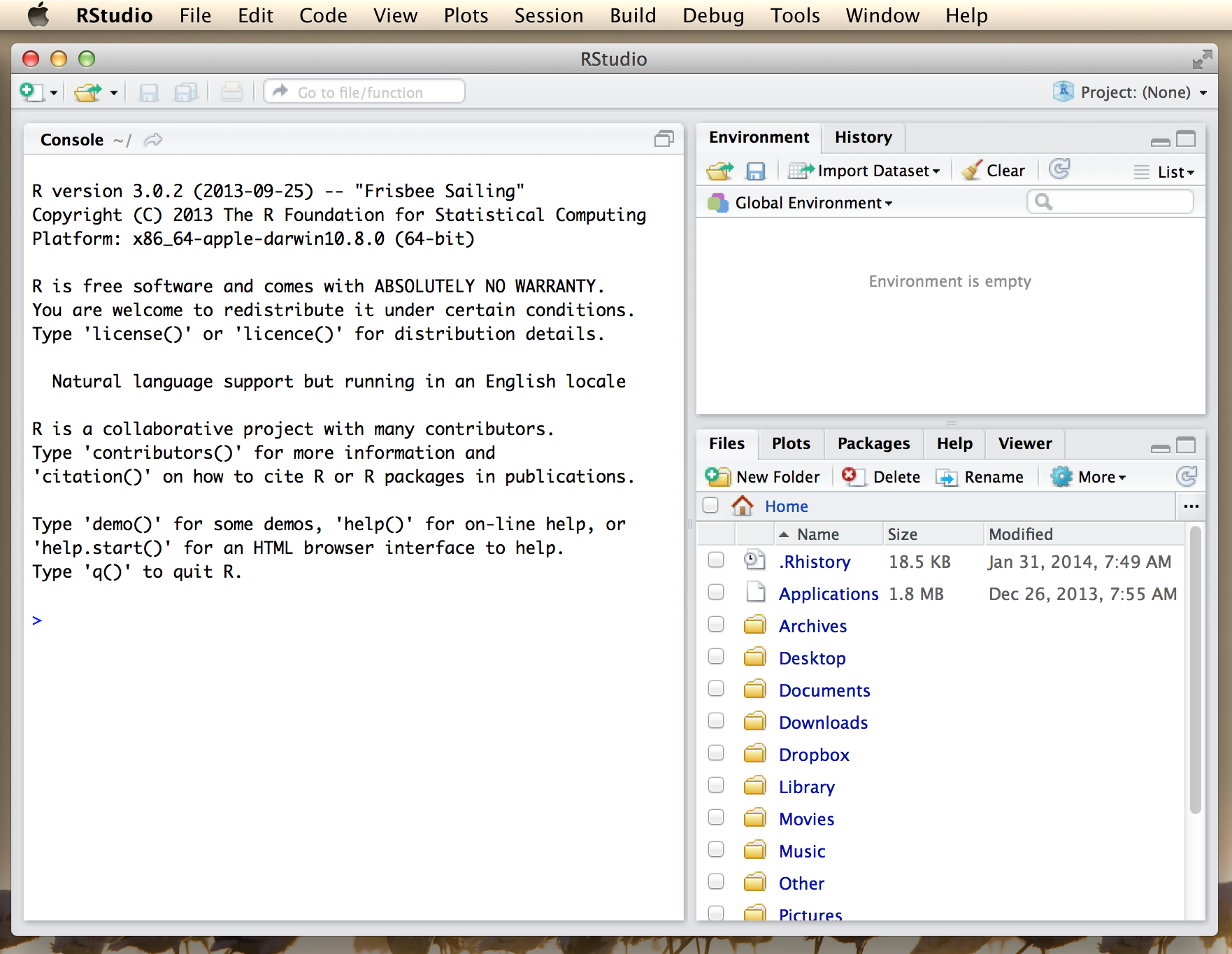
Figure 2.1: An R session in progress running through RStudio. The picture shows RStudio running on a Mac, but the Windows interface is almost identical.
The only “shortcoming” I’ve found with RStudio is that – as of this writing – it’s still a work in progress. The “problem” is that they keep improving it. New features keep turning up the more recent releases, so there’s a good chance that by the time you read this book there will be a version out that has some really neat things that weren’t in the version that I’m using now.
2.3.5 Starting up R
One way or another, regardless of what operating system you’re using and regardless of whether you’re using RStudio, or the default GUI, or even the command line, it’s time to open R and get started. When you do that, the first thing you’ll see (assuming that you’re looking at the R console, that is) is a whole lot of text that doesn’t make much sense. It should look something like this:
R version 3.0.2 (2013-09-25) -- "Frisbee Sailing"
Copyright (C) 2013 The R Foundation for Statistical Computing
Platform: x86_64-apple-darwin10.8.0 (64-bit)

R is free software and comes with ABSOLUTELY NO WARRANTY.
You are welcome to redistribute it under certain conditions.
Type 'license()' or 'licence()' for distribution details.

  Natural language support but running in an English locale

R is a collaborative project with many contributors.
Type 'contributors()' for more information and
'citation()' on how to cite R or R packages in publications.

Type 'demo()' for some demos, 'help()' for on-line help, or
'help.start()' for an HTML browser interface to help.
Type 'q()' to quit R.

>
Most of this text is pretty uninteresting, and when doing real data analysis you’ll never really pay much attention to it. The important part of it is this…
>… which has a flashing cursor next to it. That’s the command prompt. When you see this, it means that R is waiting patiently for you to do something!
2.4 Typing commands at the R console
See also: video links at the start of this chapter
One of the easiest things you can do with R is use it as a simple calculator, so it’s a good place to start. For instance, try typing 10 + 20, and hitting enter.10 When you do this, you’ve entered a command, and R will “execute” that command. What you see on screen now will be this:
> 10 + 20
[1] 30
Not a lot of surprises in this extract. But there’s a few things worth talking about, even with such a simple example. Firstly, it’s important that you understand how to read the extract. In this example, what I typed was the 10 + 20 part. I didn’t type the > symbol: that’s just the R command prompt and isn’t part of the actual command. And neither did I type the [1] 30 part. That’s what R printed out in response to my command.
Secondly, it’s important to understand how the output is formatted. Obviously, the correct answer to the sum 10 + 20 is 30, and not surprisingly R has printed that out as part of its response. But it’s also printed out this [1] part, which probably doesn’t make a lot of sense to you right now. You’re going to see that a lot. I’ll talk about what this means in a bit more detail later on, but for now you can think of [1] 30 as if R were saying “the answer to the 1st question you asked is 30.” That’s not quite the truth, but it’s close enough for now. And in any case it’s not really very interesting at the moment: we only asked R to calculate one thing, so obviously there’s only one answer printed on the screen. Later on this will change, and the [1] part will start to make a bit more sense. For now, I just don’t want you to get confused or concerned by it.
2.4.1 An important digression about formatting
Now that I’ve taught you these rules I’m going to change them pretty much immediately. That is because I want you to be able to copy code from the book directly into R if if you want to test things or conduct your own analyses. However, if you copy this kind of code (that shows the command prompt and the results) directly into R you will get an error
> 10 + 20
[1] 30
## Error: <text>:1:1: unexpected '>'
## 1: >
## ^So instead, I’m going to provide code in a slightly different format so that it looks like this…
10 + 20## [1] 30There are two main differences.
- In your console, you type after the >, but from now I I won’t show the command prompt in the book.
- In the book, output is commented out with ##, in your console it appears directly after your code.
These two differences mean that if you’re working with an electronic version of the book, you can easily copy code out of the book and into the console.
So for example if you copied the two lines of code from the book you’d get this
10 + 20## [1] 30## [1] 302.4.2 Be very careful to avoid typos
Before we go on to talk about other types of calculations that we can do with R, there’s a few other things I want to point out. The first thing is that, while R is good software, it’s still software. It’s pretty stupid, and because it’s stupid it can’t handle typos. It takes it on faith that you meant to type exactly what you did type. For example, suppose that you forgot to hit the shift key when trying to type +, and as a result your command ended up being 10 = 20 rather than 10 + 20. Here’s what happens:
10 = 20## Error in 10 = 20: invalid (do_set) left-hand side to assignmentWhat’s happened here is that R has attempted to interpret 10 = 20 as a command, and spits out an error message because the command doesn’t make any sense to it. When a human looks at this, and then looks down at his or her keyboard and sees that + and = are on the same key, it’s pretty obvious that the command was a typo. But R doesn’t know this, so it gets upset. And, if you look at it from its perspective, this makes sense. All that R “knows” is that 10 is a legitimate number, 20 is a legitimate number, and = is a legitimate part of the language too. In other words, from its perspective this really does look like the user meant to type 10 = 20, since all the individual parts of that statement are legitimate and it’s too stupid to realise that this is probably a typo. Therefore, R takes it on faith that this is exactly what you meant… it only “discovers” that the command is nonsense when it tries to follow your instructions, typo and all. And then it whinges, and spits out an error.
Even more subtle is the fact that some typos won’t produce errors at all, because they happen to correspond to “well-formed” R commands. For instance, suppose that not only did I forget to hit the shift key when trying to type 10 + 20, I also managed to press the key next to one I meant do. The resulting typo would produce the command 10 - 20. Clearly, R has no way of knowing that you meant to add 20 to 10, not subtract 20 from 10, so what happens this time is this:
10 - 20## [1] -10In this case, R produces the right answer, but to the the wrong question.
To some extent, I’m stating the obvious here, but it’s important. The people who wrote R are smart. You, the user, are smart. But R itself is dumb. And because it’s dumb, it has to be mindlessly obedient. It does exactly what you ask it to do. There is no equivalent to “autocorrect” in R, and for good reason. When doing advanced stuff – and even the simplest of statistics is pretty advanced in a lot of ways – it’s dangerous to let a mindless automaton like R try to overrule the human user. But because of this, it’s your responsibility to be careful. Always make sure you type exactly what you mean. When dealing with computers, it’s not enough to type “approximately” the right thing. In general, you absolutely must be precise in what you say to R … like all machines it is too stupid to be anything other than absurdly literal in its interpretation.
2.4.3 R is (a bit) flexible with spacing
Of course, now that I’ve been so uptight about the importance of always being precise, I should point out that there are some exceptions. Or, more accurately, there are some situations in which R does show a bit more flexibility than my previous description suggests. The first thing R is smart enough to do is ignore redundant spacing. What I mean by this is that, when I typed 10 + 20 before, I could equally have done this
10 + 20## [1] 30or this
10+20## [1] 30and I would get exactly the same answer. However, that doesn’t mean that you can insert spaces in any old place. When we looked at the startup documentation in Section 2.3.5 it suggested that you could type citation() to get some information about how to cite R. If I do so…
citation()##
## To cite R in publications use:
##
## R Core Team (2020). R: A language and environment for statistical
## computing. R Foundation for Statistical Computing, Vienna, Austria.
## URL https://www.R-project.org/.
##
## A BibTeX entry for LaTeX users is
##
## @Manual{,
## title = {R: A Language and Environment for Statistical Computing},
## author = {{R Core Team}},
## organization = {R Foundation for Statistical Computing},
## address = {Vienna, Austria},
## year = {2020},
## url = {https://www.R-project.org/},
## }
##
## We have invested a lot of time and effort in creating R, please cite it
## when using it for data analysis. See also 'citation("pkgname")' for
## citing R packages.… it tells me to cite the R manual (R Core Team 2013). Let’s see what happens when I try changing the spacing. If I insert spaces in between the word and the parentheses, or inside the parentheses themselves, then all is well. That is, either of these two commands
citation ()citation( )will produce exactly the same response. However, what I can’t do is insert spaces in the middle of the word. If I try to do this, R gets upset:
citat ion()## Error: <text>:1:7: unexpected symbol
## 1: citat ion
## ^Throughout this book I’ll vary the way I use spacing a little bit, just to give you a feel for the different ways in which spacing can be used. I’ll try not to do it too much though, since it’s generally considered to be good practice to be consistent in how you format your commands.
2.4.4 R can sometimes tell that you’re not finished yet (but not often)
One more thing I should point out. If you hit enter in a situation where it’s “obvious” to R that you haven’t actually finished typing the command, R is just smart enough to keep waiting. For example, if you type 10 + and then press enter, even R is smart enough to realise that you probably wanted to type in another number. So here’s what happens (for illustrative purposes I’m breaking my own code formatting rules in this section):
> 10+
+
and there’s a blinking cursor next to the plus sign. What this means is that R is still waiting for you to finish. It “thinks” you’re still typing your command, so it hasn’t tried to execute it yet. In other words, this plus sign is actually another command prompt. It’s different from the usual one (i.e., the > symbol) to remind you that R is going to “add” whatever you type now to what you typed last time. For example, if I then go on to type 3 and hit enter, what I get is this:
> 10 +
+ 20
[1] 30
And as far as R is concerned, this is exactly the same as if you had typed 10 + 20. Similarly, consider the citation() command that we talked about in the previous section. Suppose you hit enter after typing citation(. Once again, R is smart enough to realise that there must be more coming – since you need to add the ) character – so it waits. I can even hit enter several times and it will keep waiting:
> citation(
+
+
+ )
I’ll make use of this a lot in this book. A lot of the commands that we’ll have to type are pretty long, and they’re visually a bit easier to read if I break it up over several lines. If you start doing this yourself, you’ll eventually get yourself in trouble (it happens to us all). Maybe you start typing a command, and then you realise you’ve screwed up. For example,
> citblation(
+
+
You’d probably prefer R not to try running this command, right? If you want to get out of this situation, just hit the ‘escape’ key.11 R will return you to the normal command prompt (i.e. >) without attempting to execute the botched command.
That being said, it’s not often the case that R is smart enough to tell that there’s more coming.
For instance, in the same way that I can’t add a space in the middle of a word, I can’t hit enter in the middle of a word either. If I hit enter after typing citat I get an error, because R thinks I’m interested in an “object” called citat and can’t find it:
> citat
Error: object 'citat' not found
What about if I typed citation and hit enter? In this case we get something very odd, something that we definitely don’t want, at least at this stage. Here’s what happens:
citation
## function (package = "base", lib.loc = NULL, auto = NULL)
## {
##     dir <- system.file(package = package, lib.loc = lib.loc)
##     if (dir == "")
##         stop(gettextf("package '%s' not found", package), domain = NA)

BLAH BLAH BLAH
where the BLAH BLAH BLAH goes on for rather a long time, and you don’t know enough R yet to understand what all this gibberish actually means (of course, it doesn’t actually say BLAH BLAH BLAH - it says some other things we don’t understand or need to know that I’ve edited for length) This incomprehensible output can be quite intimidating to novice users, and unfortunately it’s very easy to forget to type the parentheses; so almost certainly you’ll do this by accident. Do not panic when this happens. Simply ignore the gibberish. As you become more experienced this gibberish will start to make sense, and you’ll find it quite handy to print this stuff out.12 But for now just try to remember to add the parentheses when typing your commands.
2.5 Doing simple calculations with R
Okay, now that we’ve discussed some of the tedious details associated with typing R commands, let’s get back to learning how to use the most powerful piece of statistical software in the world as a $2 calculator. So far, all we know how to do is addition. Clearly, a calculator that only did addition would be a bit stupid, so I should tell you about how to perform other simple calculations using R. But first, some more terminology. Addition is an example of an “operation” that you can perform (specifically, an arithmetic operation), and the operator that performs it is +. To people with a programming or mathematics background, this terminology probably feels pretty natural, but to other people it might feel like I’m trying to make something very simple (addition) sound more complicated than it is (by calling it an arithmetic operation). To some extent, that’s true: if addition was the only operation that we were interested in, it’d be a bit silly to introduce all this extra terminology. However, as we go along, we’ll start using more and more different kinds of operations, so it’s probably a good idea to get the language straight now, while we’re still talking about very familiar concepts like addition!
2.5.1 Adding, subtracting, multiplying and dividing
So, now that we have the terminology, let’s learn how to perform some arithmetic operations in R. To that end, Table 2.1 lists the operators that correspond to the basic arithmetic we learned in primary school: addition, subtraction, multiplication and division.
| operation | operator | example input | example output |
|---|---|---|---|
| addition | + |
10 + 2 | 12 |
| subtraction | - |
9 - 3 | 6 |
| multiplication | * |
5 * 5 | 25 |
| division | / |
10 / 3 | 3 |
| power | ^ |
5 ^ 2 | 25 |
As you can see, R uses fairly standard symbols to denote each of the different operations you might want to perform: addition is done using the + operator, subtraction is performed by the - operator, and so on. So if I wanted to find out what 57 times 61 is (and who wouldn’t?), I can use R instead of a calculator, like so:
57 * 61## [1] 3477So that’s handy.
2.5.2 Taking powers
The first four operations listed in Table 2.1 are things we all learned in primary school, but they aren’t the only arithmetic operations built into R. There are three other arithmetic operations that I should probably mention: taking powers, doing integer division, and calculating a modulus. Of the three, the only one that is of any real importance for the purposes of this book is taking powers, so I’ll discuss that one here: the other two are discussed in Chapter ??.
For those of you who can still remember your high school maths, this should be familiar. But for some people high school maths was a long time ago, and others of us didn’t listen very hard in high school. It’s not complicated. As I’m sure everyone will probably remember the moment they read this, the act of multiplying a number \(x\) by itself \(n\) times is called “raising \(x\) to the \(n\)-th power.” Mathematically, this is written as \(x^n\). Some values of \(n\) have special names: in particular \(x^2\) is called \(x\)-squared, and \(x^3\) is called \(x\)-cubed. So, the 4th power of 5 is calculated like this: \[ 5^4 = 5 \times 5 \times 5 \times 5 \]
One way that we could calculate \(5^4\) in R would be to type in the complete multiplication as it is shown in the equation above. That is, we could do this
5 * 5 * 5 * 5## [1] 625but it does seem a bit tedious. It would be very annoying indeed if you wanted to calculate \(5^{15}\), since the command would end up being quite long. Therefore, to make our lives easier, we use the power operator instead. When we do that, our command to calculate \(5^4\) goes like this:
5 ^ 4## [1] 625Much easier.
2.5.3 Doing calculations in the right order
Okay. At this point, you know how to take one of the most powerful pieces of statistical software in the world, and use it as a $2 calculator. And as a bonus, you’ve learned a few very basic programming concepts. That’s not nothing (you could argue that you’ve just saved yourself $2) but on the other hand, it’s not very much either. In order to use R more effectively, we need to introduce more programming concepts.
In most situations where you would want to use a calculator, you might want to do multiple calculations. R lets you do this, just by typing in longer commands.13 In fact, we’ve already seen an example of this earlier, when I typed in 5 * 5 * 5 * 5. However, let’s try a slightly different example:
1 + 2 * 4## [1] 9Clearly, this isn’t a problem for R either. However, it’s worth stopping for a second, and thinking about what R just did. Clearly, since it gave us an answer of 9 it must have multiplied 2 * 4 (to get an interim answer of 8) and then added 1 to that. But, suppose it had decided to just go from left to right: if R had decided instead to add 1+2 (to get an interim answer of 3) and then multiplied by 4, it would have come up with an answer of 12.
To answer this, you need to know the order of operations that R uses. If you remember back to your high school maths classes, it’s actually the same order that you got taught when you were at school: the “BEDMAS” order.14 That is, first calculate things inside Brackets (), then calculate Exponents ^, then Division / and Multiplication *, then Addition + and Subtraction -. So, to continue the example above, if we want to force R to calculate the 1+2 part before the multiplication, all we would have to do is enclose it in brackets:
(1 + 2) * 4 ## [1] 12This is a fairly useful thing to be able to do. The only other thing I should point out about order of operations is what to expect when you have two operations that have the same priority: that is, how does R resolve ties? For instance, multiplication and division are actually the same priority, but what should we expect when we give R a problem like 4 / 2 * 3 to solve? If it evaluates the multiplication first and then the division, it would calculate a value of two-thirds. But if it evaluates the division first it calculates a value of 6. The answer, in this case, is that R goes from left to right, so in this case the division step would come first:
4 / 2 * 3## [1] 6All of the above being said, it’s helpful to remember that brackets always come first. So, if you’re ever unsure about what order R will do things in, an easy solution is to enclose the thing you want it to do first in brackets. There’s nothing stopping you from typing (4 / 2) * 3. By enclosing the division in brackets we make it clear which thing is supposed to happen first. In this instance you wouldn’t have needed to, since R would have done the division first anyway, but when you’re first starting out it’s better to make sure R does what you want!
2.6 Storing a number as a variable
One of the most important things to be able to do in R (or any programming language, for that matter) is to store information in variables. Variables in R aren’t exactly the same thing as the variables we talked about in the last chapter on research methods, but they are similar. At a conceptual level you can think of a variable as label for a certain piece of information, or even several different pieces of information. When doing statistical analysis in R all of your data (the variables you measured in your study) will be stored as variables in R, but as well see later in the book you’ll find that you end up creating variables for other things too. However, before we delve into all the messy details of data sets and statistical analysis, let’s look at the very basics for how we create variables and work with them.
2.6.1 Variable assignment using <- and ->
Since we’ve been working with numbers so far, let’s start by creating variables to store our numbers. And since most people like concrete examples, let’s invent one. Suppose I’m trying to calculate how much money I’m going to make from this book. There’s several different numbers I might want to store. Firstly, I need to figure out how many copies I’ll sell. This isn’t exactly Harry Potter, so let’s assume I’m only going to sell one copy per student in my class. That’s 350 sales, so let’s create a variable called sales. What I want to do is assign a value to my variable sales, and that value should be 350. We do this by using the assignment operator, which is <-. Here’s how we do it:
sales <- 350When you hit enter, R doesn’t print out any output.15 It just gives you another command prompt. However, behind the scenes R has created a variable called sales and given it a value of 350. You can check that this has happened by asking R to print the variable on screen. And the simplest way to do that is to type the name of the variable and hit enter16.
sales## [1] 350So that’s nice to know. Anytime you can’t remember what R has got stored in a particular variable, you can just type the name of the variable and hit enter.
Okay, so now we know how to assign variables. Actually, there’s a bit more you should know. Firstly, one of the curious features of R is that there are several different ways of making assignments. In addition to the <- operator, we can also use -> and =, and it’s pretty important to understand the differences between them.17 Let’s start by considering ->, since that’s the easy one (we’ll discuss the use of = in Section 2.7.1. As you might expect from just looking at the symbol, it’s almost identical to <-. It’s just that the arrow (i.e., the assignment) goes from left to right. So if I wanted to define my sales variable using ->, I would write it like this:
350 -> salesThis has the same effect: and it still means that I’m only going to sell 350 copies. Sigh. Apart from this superficial difference, <- and -> are identical. In fact, as far as R is concerned, they’re actually the same operator, just in a “left form” and a “right form.”18
2.6.2 Doing calculations using variables
Okay, let’s get back to my original story. In my quest to become rich, I’ve written this textbook. To figure out how good a strategy is, I’ve started creating some variables in R. In addition to defining a sales variable that counts the number of copies I’m going to sell, I can also create a variable called royalty, indicating how much money I get per copy. Let’s say that my royalties are about $7 per book:
sales <- 350
royalty <- 7
The nice thing about variables (in fact, the whole point of having variables) is that we can do anything with a variable that we ought to be able to do with the information that it stores. That is, since R allows me to multiply 350 by 7
350 * 7## [1] 2450it also allows me to multiply sales by royalty
sales * royalty## [1] 2450As far as R is concerned, the sales * royalty command is the same as the 350 * 7 command. Not surprisingly, I can assign the output of this calculation to a new variable, which I’ll call revenue. And when we do this, the new variable revenue gets the value 2450. So let’s do that, and then get R to print out the value of revenue so that we can verify that it’s done what we asked:
revenue <- sales * royalty
revenue
## [1] 2450That’s fairly straightforward. A slightly more subtle thing we can do is reassign the value of my variable, based on its current value. For instance, suppose that one of my students (no doubt under the influence of psychotropic drugs) loves the book so much that he or she donates me an extra $550. The simplest way to capture this is by a command like this:
revenue <- revenue + 550
revenue
## [1] 3000In this calculation, R has taken the old value of revenue (i.e., 2450) and added 550 to that value, producing a value of 3000. This new value is assigned to the revenue variable, overwriting its previous value. In any case, we now know that I’m expecting to make $3000 off this. Pretty sweet, I thinks to myself. Or at least, that’s what I thinks until I do a few more calculation and work out what the implied hourly wage I’m making off this looks like.
2.6.3 Rules and conventions for naming variables
In the examples that we’ve seen so far, my variable names (sales and revenue) have just been English-language words written using lowercase letters. However, R allows a lot more flexibility when it comes to naming your variables, as the following list of rules19 illustrates:
- Variable names can only use the upper case alphabetic characters
A-Zas well as the lower case charactersa-z. You can also include numeric characters0-9in the variable name, as well as the period.or underscore_character. In other words, you can useSaL.e_sas a variable name (though I can’t think why you would want to), but you can’t useSales?. - Variable names cannot include spaces: therefore
my salesis not a valid name, butmy.salesis. - Variable names are case sensitive: that is,
Salesandsalesare different variable names. - Variable names must start with a letter or a period. You can’t use something like
_salesor1salesas a variable name. You can use.salesas a variable name if you want, but it’s not usually a good idea. By convention, variables starting with a.are used for special purposes, so you should avoid doing so. - Variable names cannot be one of the reserved keywords. These are special names that R needs to keep “safe” from us mere users, so you can’t use them as the names of variables. The keywords are:
if,else,repeat,while,function,for,in,next,break,TRUE,FALSE,NULL,Inf,NaN,NA,NA_integer_,NA_real_,NA_complex_, and finally,NA_character_. Don’t feel especially obliged to memorise these: if you make a mistake and try to use one of the keywords as a variable name, R will complain about it like the whiny little automaton it is.
In addition to those rules that R enforces, there are some informal conventions that people tend to follow when naming variables. One of them you’ve already seen: i.e., don’t use variables that start with a period. But there are several others. You aren’t obliged to follow these conventions, and there are many situations in which it’s advisable to ignore them, but it’s generally a good idea to follow them when you can:
- Use informative variable names. As a general rule, using meaningful names like
salesandrevenueis preferred over arbitrary ones likevariable1andvariable2. Otherwise it’s very hard to remember what the contents of different variables are, and it becomes hard to understand what your commands actually do. - Use short variable names. Typing is a pain and no-one likes doing it. So we much prefer to use a name like
salesover a name likesales.for.this.book.that.you.are.reading. Obviously there’s a bit of a tension between using informative names (which tend to be long) and using short names (which tend to be meaningless), so use a bit of common sense when trading off these two conventions. - Use one of the conventional naming styles for multi-word variable names. Suppose I want to name a variable that stores “my new salary.” Obviously I can’t include spaces in the variable name, so how should I do this? There are three different conventions that you sometimes see R users employing. Firstly, you can separate the words using periods, which would give you
my.new.salaryas the variable name. Alternatively, you could separate words using underscores, as inmy_new_salary. Finally, you could use capital letters at the beginning of each word (except the first one), which gives youmyNewSalaryas the variable name. I don’t think there’s any strong reason to prefer one over the other,20 but it’s important to be consistent.
2.7 Using functions to do calculations
The symbols +, -, * and so on are examples of operators. As we’ve seen, you can do quite a lot of calculations just by using these operators. However, in order to do more advanced calculations (and later on, to do actual statistics), you’re going to need to start using functions.21 I’ll talk in more detail about functions and how they work in Section ??, but for now let’s just dive in and use a few. To get started, suppose I wanted to take the square root of 225. The square root, in case your high school maths is a bit rusty, is just the opposite of squaring a number. So, for instance, since “5 squared is 25” I can say that “5 is the square root of 25.” The usual notation for this is
\[ \sqrt{25} = 5 \]
though sometimes you’ll also see it written like this \(25^{0.5} = 5.\) This second way of writing it is kind of useful to “remind” you of the mathematical fact that “square root of \(x\)” is actually the same as “raising \(x\) to the power of 0.5.” Personally, I’ve never found this to be terribly meaningful psychologically, though I have to admit it’s quite convenient mathematically. Anyway, it’s not important. What is important is that you remember what a square root is, since we’re going to need it later on.
To calculate the square root of 25, I can do it in my head pretty easily, since I memorised my multiplication tables when I was a kid. It gets harder when the numbers get bigger, and pretty much impossible if they’re not whole numbers. This is where something like R comes in very handy. Let’s say I wanted to calculate \(\sqrt{225}\), the square root of 225. There’s two ways I could do this using R. Firstly, since the square root of 255 is the same thing as raising 225 to the power of 0.5, I could use the power operator ^, just like we did earlier:
225 ^ 0.5## [1] 15However, there’s a second way that we can do this, since R also provides a square root function, sqrt(). To calculate the square root of 255 using this function, what I do is insert the number 225 in the parentheses. That is, the command I type is this:
sqrt( 225 )## [1] 15and as you might expect from our previous discussion, the spaces in between the parentheses are purely cosmetic. I could have typed sqrt(225) or sqrt( 225 ) and gotten the same result. When we use a function to do something, we generally refer to this as calling the function, and the values that we type into the function (there can be more than one) are referred to as the arguments of that function.
Obviously, the sqrt() function doesn’t really give us any new functionality, since we already knew how to do square root calculations by using the power operator ^, though I do think it looks nicer when we use sqrt(). However, there are lots of other functions in R: in fact, almost everything of interest that I’ll talk about in this book is an R function of some kind. For example, one function that we will need to use in this book is the absolute value function. Compared to the square root function, it’s extremely simple: it just converts negative numbers to positive numbers, and leaves positive numbers alone. Mathematically, the absolute value of \(x\) is written \(|x|\) or sometimes \(\mbox{abs}(x)\). Calculating absolute values in R is pretty easy, since R provides the abs() function that you can use for this purpose. When you feed it a positive number…
abs( 21 )## [1] 21the absolute value function does nothing to it at all. But when you feed it a negative number, it spits out the positive version of the same number, like this:
abs( -13 )## [1] 13In all honesty, there’s nothing that the absolute value function does that you couldn’t do just by looking at the number and erasing the minus sign if there is one. However, there’s a few places later in the book where we have to use absolute values, so I thought it might be a good idea to explain the meaning of the term early on.
Before moving on, it’s worth noting that – in the same way that R allows us to put multiple operations together into a longer command, like 1 + 2*4 for instance – it also lets us put functions together and even combine functions with operators if we so desire. For example, the following is a perfectly legitimate command:
sqrt( 1 + abs(-8) )## [1] 3When R executes this command, starts out by calculating the value of abs(-8), which produces an intermediate value of 8. Having done so, the command simplifies to sqrt( 1 + 8 ). To solve the square root22 it first needs to add 1 + 8 to get 9, at which point it evaluates sqrt(9), and so it finally outputs a value of 3.
2.7.1 Function arguments, their names and their defaults
There’s two more fairly important things that you need to understand about how functions work in R, and that’s the use of “named” arguments, and default values" for arguments. Not surprisingly, that’s not to say that this is the last we’ll hear about how functions work, but they are the last things we desperately need to discuss in order to get you started. To understand what these two concepts are all about, I’ll introduce another function. The round() function can be used to round some value to the nearest whole number. For example, I could type this:
round( 3.1415 )## [1] 3Pretty straightforward, really. However, suppose I only wanted to round it to two decimal places: that is, I want to get 3.14 as the output. The round() function supports this, by allowing you to input a second argument to the function that specifies the number of decimal places that you want to round the number to. In other words, I could do this:
round( 3.14165, 2 )## [1] 3.14What’s happening here is that I’ve specified two arguments: the first argument is the number that needs to be rounded (i.e., 3.1415), the second argument is the number of decimal places that it should be rounded to (i.e., 2), and the two arguments are separated by a comma. In this simple example, it’s quite easy to remember which one argument comes first and which one comes second, but for more complicated functions this is not easy. Fortunately, most R functions make use of argument names. For the round() function, for example the number that needs to be rounded is specified using the x argument, and the number of decimal points that you want it rounded to is specified using the digits argument. Because we have these names available to us, we can specify the arguments to the function by name. We do so like this:
round( x = 3.1415, digits = 2 )## [1] 3.14Notice that this is kind of similar in spirit to variable assignment (Section 2.6), except that I used = here, rather than <-. In both cases we’re specifying specific values to be associated with a label. However, there are some differences between what I was doing earlier on when creating variables, and what I’m doing here when specifying arguments, and so as a consequence it’s important that you use = in this context.
As you can see, specifying the arguments by name involves a lot more typing, but it’s also a lot easier to read. Because of this, the commands in this book will usually specify arguments by name,23 since that makes it clearer to you what I’m doing. However, one important thing to note is that when specifying the arguments using their names, it doesn’t matter what order you type them in. But if you don’t use the argument names, then you have to input the arguments in the correct order. In other words, these three commands all produce the same output…
round( 3.14165, 2 )## [1] 3.14round( x = 3.1415, digits = 2 )## [1] 3.14round( digits = 2, x = 3.1415 )## [1] 3.14but this one does not…
round( 2, 3.14165 )## [1] 2How do you find out what the correct order is? There’s a few different ways, but the easiest one is to look at the help documentation for the function (see Section 2.27. However, if you’re ever unsure, it’s probably best to actually type in the argument name.
Okay, so that’s the first thing I said you’d need to know: argument names. The second thing you need to know about is default values. Notice that the first time I called the round() function I didn’t actually specify the digits argument at all, and yet R somehow knew that this meant it should round to the nearest whole number. How did that happen? The answer is that the digits argument has a default value of 0, meaning that if you decide not to specify a value for digits then R will act as if you had typed digits = 0. This is quite handy: the vast majority of the time when you want to round a number you want to round it to the nearest whole number, and it would be pretty annoying to have to specify the digits argument every single time. On the other hand, sometimes you actually do want to round to something other than the nearest whole number, and it would be even more annoying if R didn’t allow this! Thus, by having digits = 0 as the default value, we get the best of both worlds.
2.8 Letting RStudio help you with your commands
Time for a bit of a digression. At this stage you know how to type in basic commands, including how to use R functions. And it’s probably beginning to dawn on you that there are a lot of R functions, all of which have their own arguments. You’re probably also worried that you’re going to have to remember all of them! Thankfully, it’s not that bad. In fact, very few data analysts bother to try to remember all the commands. What they really do is use tricks to make their lives easier. The first (and arguably most important one) is to use the internet. If you don’t know how a particular R function works, Google it. Second, you can look up the R help documentation. I’ll talk more about these two tricks in Section 2.27. But right now I want to call your attention to a couple of simple tricks that RStudio makes available to you.
2.8.1 Autocomplete using “tab”
The first thing I want to call your attention to is the autocomplete ability in RStudio.24
Let’s stick to our example above and assume that what you want to do is to round a number. This time around, start typing the name of the function that you want, and then hit the “tab” key. RStudio will then display a little window like the one shown in Figure 2.2. In this figure, I’ve typed the letters ro at the command line, and then hit tab. The window has two panels. On the left, there’s a list of variables and functions that start with the letters that I’ve typed shown in black text, and some grey text that tells you where that variable/function is stored. Ignore the grey text for now: it won’t make much sense to you until we’ve talked about packages in Section 2.17. In Figure 2.2 you can see that there’s quite a few things that start with the letters ro: there’s something called rock, something called round, something called round.Date and so on. The one we want is round, but if you’re typing this yourself you’ll notice that when you hit the tab key the window pops up with the top entry (i.e., rock) highlighted. You can use the up and down arrow keys to select the one that you want. Or, if none of the options look right to you, you can hit the escape key (“esc”) or the left arrow key to make the window go away.
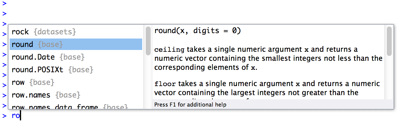
Figure 2.2: Start typing the name of a function or a variable, and hit the “tab” key. RStudio brings up a little dialog box like this one that lets you select the one you want, and even prints out a little information about it.
In our case, the thing we want is the round option, so we’ll select that. When you do this, you’ll see that the panel on the right changes. Previously, it had been telling us something about the rock data set (i.e., “Measurements on 48 rock samples…”) that is distributed as part of R. But when we select round, it displays information about the round() function, exactly as it is shown in Figure 2.2. This display is really handy. The very first thing it says is round(x, digits = 0): what this is telling you is that the round() function has two arguments. The first argument is called x, and it doesn’t have a default value. The second argument is digits, and it has a default value of 0. In a lot of situations, that’s all the information you need. But RStudio goes a bit further, and provides some additional information about the function underneath. Sometimes that additional information is very helpful, sometimes it’s not: RStudio pulls that text from the R help documentation, and my experience is that the helpfulness of that documentation varies wildly. Anyway, if you’ve decided that round() is the function that you want to use, you can hit the right arrow or the enter key, and RStudio will finish typing the rest of the function name for you.
The RStudio autocomplete tool works slightly differently if you’ve already got the name of the function typed and you’re now trying to type the arguments. For instance, suppose I’ve typed round( into the console, and then I hit tab. RStudio is smart enough to recognise that I already know the name of the function that I want, because I’ve already typed it! Instead, it figures that what I’m interested in is the arguments to that function. So that’s what pops up in the little window. You can see this in Figure 2.3. Again, the window has two panels, and you can interact with this window in exactly the same way that you did with the window shown in Figure 2.2. On the left hand panel, you can see a list of the argument names. On the right hand side, it displays some information about what the selected argument does.
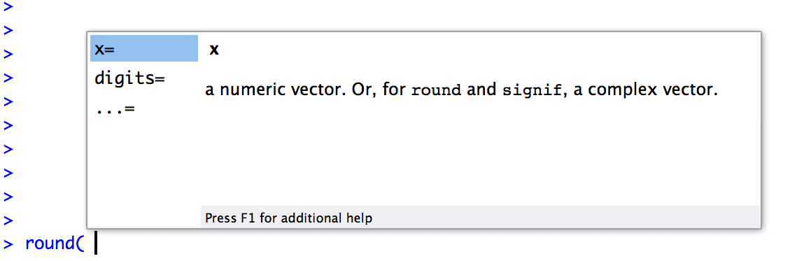
Figure 2.3: If you’ve typed the name of a function already along with the left parenthesis and then hit the “tab” key, RStudio brings up a different window to the one shown above. This one lists all the arguments to the function on the left, and information about each argument on the right.
2.8.2 Browsing your command history
One thing that R does automatically is keep track of your “command history.” That is, it remembers all the commands that you’ve previously typed. You can access this history in a few different ways. The simplest way is to use the up and down arrow keys. If you hit the up key, the R console will show you the most recent command that you’ve typed. Hit it again, and it will show you the command before that. If you want the text on the screen to go away, hit escape25 Using the up and down keys can be really handy if you’ve typed a long command that had one typo in it. Rather than having to type it all again from scratch, you can use the up key to bring up the command and fix it.
The second way to get access to your command history is to look at the history panel in RStudio. On the upper right hand side of the RStudio window you’ll see a tab labelled “History.” Click on that, and you’ll see a list of all your recent commands displayed in that panel: it should look something like Figure 2.4. If you double click on one of the commands, it will be copied to the R console. (You can achieve the same result by selecting the command you want with the mouse and then clicking the “To Console” button).26
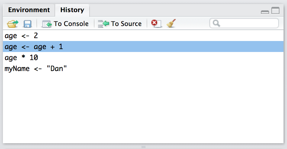
Figure 2.4: The history panel is located in the top right hand side of the RStudio window. Click on the word “History” and it displays this panel.
2.9 Storing many numbers as a vector
At this point we’ve covered functions in enough detail to get us safely through the next couple of chapters (with one small exception: see Section 2.26, so let’s return to our discussion of variables. When I introduced variables in Section 2.6 I showed you how we can use variables to store a single number. In this section, we’ll extend this idea and look at how to store multiple numbers within the one variable. In R, the name for a variable that can store multiple values is a vector. So let’s create one.
2.9.1 Creating a vector
Let’s stick to my silly “get rich quick by textbook writing” example. Suppose the textbook company (if I actually had one, that is) sends me sales data on a monthly basis. Since my class start in late February, we might expect most of the sales to occur towards the start of the year. Let’s suppose that I have 100 sales in February, 200 sales in March and 50 sales in April, and no other sales for the rest of the year. What I would like to do is have a variable – let’s call it sales.by.month – that stores all this sales data. The first number stored should be 0 since I had no sales in January, the second should be 100, and so on. The simplest way to do this in R is to use the combine function, c(). To do so, all we have to do is type all the numbers you want to store in a comma separated list, like this:27
sales.by.month <- c(0, 100, 200, 50, 0, 0, 0, 0, 0, 0, 0, 0)
sales.by.month
## [1] 0 100 200 50 0 0 0 0 0 0 0 0To use the correct terminology here, we have a single variable here called sales.by.month: this variable is a vector that consists of 12 elements.
2.9.2 A handy digression
Now that we’ve learned how to put information into a vector, the next thing to understand is how to pull that information back out again. However, before I do so it’s worth taking a slight detour. If you’ve been following along, typing all the commands into R yourself, it’s possible that the output that you saw when we printed out the sales.by.month vector was slightly different to what I showed above. This would have happened if the window (or the RStudio panel) that contains the R console is really, really narrow. If that were the case, you might have seen output that looks something like this:
sales.by.month## [1] 0 100 200 50
## [5] 0 0 0 0
## [9] 0 0 0 0Because there wasn’t much room on the screen, R has printed out the results over three lines. But that’s not the important thing to notice. The important point is that the first line has a [1] in front of it, whereas the second line starts with [5] and the third with [9]. It’s pretty clear what’s happening here. For the first row, R has printed out the 1st element through to the 4th element, so it starts that row with a [1]. For the second row, R has printed out the 5th element of the vector through to the 8th one, and so it begins that row with a [5] so that you can tell where it’s up to at a glance. It might seem a bit odd to you that R does this, but in some ways it’s a kindness, especially when dealing with larger data sets!
2.9.3 Getting information out of vectors
To get back to the main story, let’s consider the problem of how to get information out of a vector. At this point, you might have a sneaking suspicion that the answer has something to do with the [1] and [9] things that R has been printing out. And of course you are correct. Suppose I want to pull out the February sales data only. February is the second month of the year, so let’s try this:
sales.by.month[2]## [1] 100Yep, that’s the February sales all right. But there’s a subtle detail to be aware of here: notice that R outputs [1] 100, not [2] 100. This is because R is being extremely literal. When we typed in sales.by.month[2], we asked R to find exactly one thing, and that one thing happens to be the second element of our sales.by.month vector. So, when it outputs [1] 100 what R is saying is that the first number that we just asked for is 100. This behaviour makes more sense when you realise that we can use this trick to create new variables. For example, I could create a february.sales variable like this:
february.sales <- sales.by.month[2]
february.sales
## [1] 100Obviously, the new variable february.sales should only have one element and so when I print it out this new variable, the R output begins with a [1] because 100 is the value of the first (and only) element of february.sales. The fact that this also happens to be the value of the second element of sales.by.month is irrelevant. We’ll pick this topic up again shortly (Section 2.12).
2.9.4 Altering the elements of a vector
Sometimes you’ll want to change the values stored in a vector. Imagine my surprise when the publisher rings me up to tell me that the sales data for May are wrong. There were actually an additional 25 books sold in May, but there was an error or something so they hadn’t told me about it. How can I fix my sales.by.month variable? One possibility would be to assign the whole vector again from the beginning, using c(). But that’s a lot of typing. Also, it’s a little wasteful: why should R have to redefine the sales figures for all 12 months, when only the 5th one is wrong? Fortunately, we can tell R to change only the 5th element, using this trick:
sales.by.month[5] <- 25
sales.by.month
## [1] 0 100 200 50 25 0 0 0 0 0 0 0Another way to edit variables is to use the edit() or fix() functions. I won’t discuss them in detail right now, but you can check them out on your own.
2.9.5 Useful things to know about vectors
Before moving on, I want to mention a couple of other things about vectors. Firstly, you often find yourself wanting to know how many elements there are in a vector (usually because you’ve forgotten). You can use the length() function to do this. It’s quite straightforward:
length( x = sales.by.month )## [1] 12Secondly, you often want to alter all of the elements of a vector at once. For instance, suppose I wanted to figure out how much money I made in each month. Since I’m earning an exciting $7 per book (no seriously, that’s actually pretty close to what authors get on the very expensive textbooks that you’re expected to purchase), what I want to do is multiply each element in the sales.by.month vector by 7. R makes this pretty easy, as the following example shows:
sales.by.month * 7## [1] 0 700 1400 350 175 0 0 0 0 0 0 0In other words, when you multiply a vector by a single number, all elements in the vector get multiplied. The same is true for addition, subtraction, division and taking powers. So that’s neat. On the other hand, suppose I wanted to know how much money I was making per day, rather than per month. Since not every month has the same number of days, I need to do something slightly different. Firstly, I’ll create two new vectors:
days.per.month <- c(31, 28, 31, 30, 31, 30, 31, 31, 30, 31, 30, 31)
profit <- sales.by.month * 7
Obviously, the profit variable is the same one we created earlier, and the days.per.month variable is pretty straightforward. What I want to do is divide every element of profit by the corresponding element of days.per.month. Again, R makes this pretty easy:
profit / days.per.month## [1] 0.000000 25.000000 45.161290 11.666667 5.645161 0.000000 0.000000
## [8] 0.000000 0.000000 0.000000 0.000000 0.000000I still don’t like all those zeros, but that’s not what matters here. Notice that the second element of the output is 25, because R has divided the second element of profit (i.e. 700) by the second element of days.per.month (i.e. 28). Similarly, the third element of the output is equal to 1400 divided by 31, and so on. We’ll talk more about calculations involving vectors later on (and in particular a thing called the “recycling rule”; Section ??), but that’s enough detail for now.
2.10 Storing text data
A lot of the time your data will be numeric in nature, but not always. Sometimes your data really needs to be described using text, not using numbers. To address this, we need to consider the situation where our variables store text. To create a variable that stores the word “hello,” we can type this:
greeting <- "hello"
greeting
## [1] "hello"When interpreting this, it’s important to recognise that the quote marks here aren’t part of the string itself. They’re just something that we use to make sure that R knows to treat the characters that they enclose as a piece of text data, known as a character string. In other words, R treats "hello" as a string containing the word “hello”; but if I had typed hello instead, R would go looking for a variable by that name! You can also use 'hello' to specify a character string.
Okay, so that’s how we store the text. Next, it’s important to recognise that when we do this, R stores the entire word "hello" as a single element: our greeting variable is not a vector of five different letters. Rather, it has only the one element, and that element corresponds to the entire character string "hello". To illustrate this, if I actually ask R to find the first element of greeting, it prints the whole string:
greeting[1]## [1] "hello"Of course, there’s no reason why I can’t create a vector of character strings. For instance, if we were to continue with the example of my attempts to look at the monthly sales data for my book, one variable I might want would include the names of all 12 months.28 To do so, I could type in a command like this
months <- c("January", "February", "March", "April", "May", "June",
            "July", "August", "September", "October", "November",
            "December")
This is a character vector containing 12 elements, each of which is the name of a month. So if I wanted R to tell me the name of the fourth month, all I would do is this:
months[4]## [1] "April"2.10.1 Working with text
Working with text data is somewhat more complicated than working with numeric data, and I discuss some of the basic ideas in Section ??, but for purposes of the current chapter we only need this bare bones sketch. The only other thing I want to do before moving on is show you an example of a function that can be applied to text data. So far, most of the functions that we have seen (i.e., sqrt(), abs() and round()) only make sense when applied to numeric data (e.g., you can’t calculate the square root of “hello”), and we’ve seen one function that can be applied to pretty much any variable or vector (i.e., length()). So it might be nice to see an example of a function that can be applied to text.
The function I’m going to introduce you to is called nchar(), and what it does is count the number of individual characters that make up a string. Recall earlier that when we tried to calculate the length() of our greeting variable it returned a value of 1: the greeting variable contains only the one string, which happens to be "hello". But what if I want to know how many letters there are in the word? Sure, I could count them, but that’s boring, and more to the point it’s a terrible strategy if what I wanted to know was the number of letters in War and Peace. That’s where the nchar() function is helpful:
nchar( x = greeting )## [1] 5That makes sense, since there are in fact 5 letters in the string "hello". Better yet, you can apply nchar() to whole vectors. So, for instance, if I want R to tell me how many letters there are in the names of each of the 12 months, I can do this:
nchar( x = months )## [1] 7 8 5 5 3 4 4 6 9 7 8 8So that’s nice to know. The nchar() function can do a bit more than this, and there’s a lot of other functions that you can do to extract more information from text or do all sorts of fancy things. However, the goal here is not to teach any of that! The goal right now is just to see an example of a function that actually does work when applied to text.
2.11 Storing “true or false” data
Time to move onto a third kind of data. A key concept in that a lot of R relies on is the idea of a logical value. A logical value is an assertion about whether something is true or false. This is implemented in R in a pretty straightforward way. There are two logical values, namely TRUE and FALSE. Despite the simplicity, a logical values are very useful things. Let’s see how they work.
2.11.1 Assessing mathematical truths
In George Orwell’s classic book 1984, one of the slogans used by the totalitarian Party was “two plus two equals five,” the idea being that the political domination of human freedom becomes complete when it is possible to subvert even the most basic of truths. It’s a terrifying thought, especially when the protagonist Winston Smith finally breaks down under torture and agrees to the proposition. “Man is infinitely malleable,” the book says. I’m pretty sure that this isn’t true of humans29 but it’s definitely not true of R. R is not infinitely malleable. It has rather firm opinions on the topic of what is and isn’t true, at least as regards basic mathematics. If I ask it to calculate 2 + 2, it always gives the same answer, and it’s not bloody 5:
2 + 2## [1] 4Of course, so far R is just doing the calculations. I haven’t asked it to explicitly assert that \(2+2 = 4\) is a true statement. If I want R to make an explicit judgement, I can use a command like this:
2 + 2 == 4## [1] TRUEWhat I’ve done here is use the equality operator, ==, to force R to make a “true or false” judgement.30 Okay, let’s see what R thinks of the Party slogan:
2+2 == 5## [1] FALSEBooyah! Freedom and ponies for all! Or something like that. Anyway, it’s worth having a look at what happens if I try to force R to believe that two plus two is five by making an assignment statement like 2 + 2 = 5 or 2 + 2 <- 5. When I do this, here’s what happens:
2 + 2 = 5## Error in 2 + 2 = 5: target of assignment expands to non-language objectR doesn’t like this very much. It recognises that 2 + 2 is not a variable (that’s what the “non-language object” part is saying), and it won’t let you try to “reassign” it. While R is pretty flexible, and actually does let you do some quite remarkable things to redefine parts of R itself, there are just some basic, primitive truths that it refuses to give up. It won’t change the laws of addition, and it won’t change the definition of the number 2.
That’s probably for the best.
2.11.2 Logical operations
So now we’ve seen logical operations at work, but so far we’ve only seen the simplest possible example. You probably won’t be surprised to discover that we can combine logical operations with other operations and functions in a more complicated way, like this:
3*3 + 4*4 == 5*5## [1] TRUEor this
sqrt( 25 ) == 5## [1] TRUENot only that, but as Table 2.2 illustrates, there are several other logical operators that you can use, corresponding to some basic mathematical concepts.
| operation | operator | example input | answer |
|---|---|---|---|
| less than | < | 2 < 3 | TRUE |
| less than or equal to | <= | 2 <= 2 | TRUE |
| greater than | > | 2 > 3 | FALSE |
| greater than or equal to | >= | 2 >= 2 | TRUE |
| equal to | == | 2 == 3 | FALSE |
| not equal to | != | 2 != 3 | TRUE |
Hopefully these are all pretty self-explanatory: for example, the less than operator < checks to see if the number on the left is less than the number on the right. If it’s less, then R returns an answer of TRUE:
99 < 100## [1] TRUEbut if the two numbers are equal, or if the one on the right is larger, then R returns an answer of FALSE, as the following two examples illustrate:
100 < 100## [1] FALSE100 < 99## [1] FALSEIn contrast, the less than or equal to operator <= will do exactly what it says. It returns a value of TRUE if the number of the left hand side is less than or equal to the number on the right hand side. So if we repeat the previous two examples using <=, here’s what we get:
100 <= 100## [1] TRUE100 <= 99## [1] FALSEAnd at this point I hope it’s pretty obvious what the greater than operator > and the greater than or equal to operator >= do! Next on the list of logical operators is the not equal to operator != which – as with all the others – does what it says it does. It returns a value of TRUE when things on either side are not identical to each other. Therefore, since \(2+2\) isn’t equal to \(5\), we get:
2 + 2 != 5## [1] TRUEWe’re not quite done yet. There are three more logical operations that are worth knowing about, listed in Table 2.3.
| operation | operator | example input | answer |
|---|---|---|---|
| not | ! | !(1==1) | FALSE |
| or | | | (1==1) | (2==3) | TRUE |
| and | & | (1==1) & (2==3) | FALSE |
These are the not operator !, the and operator &, and the or operator |. Like the other logical operators, their behaviour is more or less exactly what you’d expect given their names. For instance, if I ask you to assess the claim that “either \(2+2 = 4\) or \(2+2 = 5\)” you’d say that it’s true. Since it’s an “either-or” statement, all we need is for one of the two parts to be true. That’s what the | operator does:
(2+2 == 4) | (2+2 == 5)## [1] TRUEOn the other hand, if I ask you to assess the claim that “both \(2+2 = 4\) and \(2+2 = 5\)” you’d say that it’s false. Since this is an and statement we need both parts to be true. And that’s what the & operator does:
(2+2 == 4) & (2+2 == 5)## [1] FALSEFinally, there’s the not operator, which is simple but annoying to describe in English. If I ask you to assess my claim that “it is not true that \(2+2 = 5\)” then you would say that my claim is true; because my claim is that “\(2+2 = 5\) is false.” And I’m right. If we write this as an R command we get this:
! (2+2 == 5)## [1] TRUEIn other words, since 2+2 == 5 is a FALSE statement, it must be the case that !(2+2 == 5) is a TRUE one. Essentially, what we’ve really done is claim that “not false” is the same thing as “true.” Obviously, this isn’t really quite right in real life. But R lives in a much more black or white world: for R everything is either true or false. No shades of gray are allowed. We can actually see this much more explicitly, like this:
! FALSE## [1] TRUEOf course, in our \(2+2 = 5\) example, we didn’t really need to use “not” ! and “equals to” == as two separate operators. We could have just used the “not equals to” operator != like this:
2+2 != 5## [1] TRUEBut there are many situations where you really do need to use the ! operator. We’ll see some later on.31
2.11.3 Storing and using logical data
Up to this point, I’ve introduced numeric data (in Sections 2.6 and 2.9) and character data (in Section 2.10). So you might not be surprised to discover that these TRUE and FALSE values that R has been producing are actually a third kind of data, called logical data. That is, when I asked R if 2 + 2 == 5 and it said [1] FALSE in reply, it was actually producing information that we can store in variables. For instance, I could create a variable called is.the.Party.correct, which would store R’s opinion:
is.the.Party.correct <- 2 + 2 == 5
is.the.Party.correct
## [1] FALSEAlternatively, you can assign the value directly, by typing TRUE or FALSE in your command. Like this:
is.the.Party.correct <- FALSE
is.the.Party.correct
## [1] FALSEBetter yet, because it’s kind of tedious to type TRUE or FALSE over and over again, R provides you with a shortcut: you can use T and F instead (but it’s case sensitive: t and f won’t work).32 So this works:
is.the.Party.correct <- F
is.the.Party.correct
## [1] FALSEbut this doesn’t:
is.the.Party.correct <- f## Error in eval(expr, envir, enclos): object 'f' not found2.11.4 Vectors of logicals
The next thing to mention is that you can store vectors of logical values in exactly the same way that you can store vectors of numbers (Section 2.9) and vectors of text data (Section 2.10). Again, we can define them directly via the c() function, like this:
x <- c(TRUE, TRUE, FALSE)
x
## [1] TRUE TRUE FALSEor you can produce a vector of logicals by applying a logical operator to a vector. This might not make a lot of sense to you, so let’s unpack it slowly. First, let’s suppose we have a vector of numbers (i.e., a “non-logical vector”). For instance, we could use the sales.by.month vector that we were using in Section 2.9. Suppose I wanted R to tell me, for each month of the year, whether I actually sold a book in that month. I can do that by typing this:
sales.by.month > 0## [1] FALSE TRUE TRUE TRUE TRUE FALSE FALSE FALSE FALSE FALSE FALSE
## [12] FALSEand again, I can store this in a vector if I want, as the example below illustrates:
any.sales.this.month <- sales.by.month > 0
any.sales.this.month
## [1] FALSE TRUE TRUE TRUE TRUE FALSE FALSE FALSE FALSE FALSE FALSE
## [12] FALSEIn other words, any.sales.this.month is a logical vector whose elements are TRUE only if the corresponding element of sales.by.month is greater than zero. For instance, since I sold zero books in January, the first element is FALSE.
2.11.5 Applying logical operation to text
In a moment (Section 2.12) I’ll show you why these logical operations and logical vectors are so handy, but before I do so I want to very briefly point out that you can apply them to text as well as to logical data. It’s just that we need to be a bit more careful in understanding how R interprets the different operations. In this section I’ll talk about how the equal to operator == applies to text, since this is the most important one. Obviously, the not equal to operator != gives the exact opposite answers to == so I’m implicitly talking about that one too, but I won’t give specific commands showing the use of !=. As for the other operators, I’ll defer a more detailed discussion of this topic to Section ??.
Okay, let’s see how it works. In one sense, it’s very simple. For instance, I can ask R if the word "cat" is the same as the word "dog", like this:
"cat" == "dog"## [1] FALSEThat’s pretty obvious, and it’s good to know that even R can figure that out. Similarly, R does recognise that a "cat" is a "cat":
"cat" == "cat"## [1] TRUEAgain, that’s exactly what we’d expect. However, what you need to keep in mind is that R is not at all tolerant when it comes to grammar and spacing. If two strings differ in any way whatsoever, R will say that they’re not equal to each other, as the following examples indicate:
" cat" == "cat"## [1] FALSE"cat" == "CAT"## [1] FALSE"cat" == "c a t"## [1] FALSE2.12 Indexing vectors
One last thing to add before finishing up this chapter. So far, whenever I’ve had to get information out of a vector, all I’ve done is typed something like months[4]; and when I do this R prints out the fourth element of the months vector. In this section, I’ll show you two additional tricks for getting information out of the vector.
2.12.1 Extracting multiple elements
One very useful thing we can do is pull out more than one element at a time. In the previous example, we only used a single number (i.e., 2) to indicate which element we wanted. Alternatively, we can use a vector. So, suppose I wanted the data for February, March and April. What I could do is use the vector c(2,3,4) to indicate which elements I want R to pull out. That is, I’d type this:
sales.by.month[ c(2,3,4) ]## [1] 100 200 50Notice that the order matters here. If I asked for the data in the reverse order (i.e., April first, then March, then February) by using the vector c(4,3,2), then R outputs the data in the reverse order:
sales.by.month[ c(4,3,2) ]## [1] 50 200 100A second thing to be aware of is that R provides you with handy shortcuts for very common situations. For instance, suppose that I wanted to extract everything from the 2nd month through to the 8th month. One way to do this is to do the same thing I did above, and use the vector c(2,3,4,5,6,7,8) to indicate the elements that I want. That works just fine
sales.by.month[ c(2,3,4,5,6,7,8) ]## [1] 100 200 50 25 0 0 0but it’s kind of a lot of typing. To help make this easier, R lets you use 2:8 as shorthand for c(2,3,4,5,6,7,8), which makes things a lot simpler. First, let’s just check that this is true:
2:8## [1] 2 3 4 5 6 7 8Next, let’s check that we can use the 2:8 shorthand as a way to pull out the 2nd through 8th elements of sales.by.months:
sales.by.month[2:8]## [1] 100 200 50 25 0 0 0So that’s kind of neat.
2.12.2 Logical indexing
At this point, I can introduce an extremely useful tool called logical indexing. In the last section, I created a logical vector any.sales.this.month, whose elements are TRUE for any month in which I sold at least one book, and FALSE for all the others. However, that big long list of TRUEs and FALSEs is a little bit hard to read, so what I’d like to do is to have R select the names of the months for which I sold any books. Earlier on, I created a vector months that contains the names of each of the months. This is where logical indexing is handy. What I need to do is this:
months[ sales.by.month > 0 ]## [1] "February" "March" "April" "May"To understand what’s happening here, it’s helpful to notice that sales.by.month > 0 is the same logical expression that we used to create the any.sales.this.month vector in the last section. In fact, I could have just done this:
months[ any.sales.this.month ]## [1] "February" "March" "April" "May"and gotten exactly the same result. In order to figure out which elements of months to include in the output, what R does is look to see if the corresponding element in any.sales.this.month is TRUE. Thus, since element 1 of any.sales.this.month is FALSE, R does not include "January" as part of the output; but since element 2 of any.sales.this.month is TRUE, R does include "February" in the output. Note that there’s no reason why I can’t use the same trick to find the actual sales numbers for those months. The command to do that would just be this:
sales.by.month [ sales.by.month > 0 ]## [1] 100 200 50 25In fact, we can do the same thing with text. Here’s an example. Suppose that – to continue the saga of the textbook sales – I later find out that the bookshop only had sufficient stocks for a few months of the year. They tell me that early in the year they had "high" stocks, which then dropped to "low" levels, and in fact for one month they were "out" of copies of the book for a while before they were able to replenish them. Thus I might have a variable called stock.levels which looks like this:
stock.levels<-c("high", "high", "low", "out", "out", "high",
                "high", "high", "high", "high", "high", "high")

stock.levels
## [1] "high" "high" "low" "out" "out" "high" "high" "high" "high" "high"
## [11] "high" "high"Thus, if I want to know the months for which the bookshop was out of my book, I could apply the logical indexing trick, but with the character vector stock.levels, like this:
months[stock.levels == "out"]## [1] "April" "May"Alternatively, if I want to know when the bookshop was either low on copies or out of copies, I could do this:
months[stock.levels == "out" | stock.levels == "low"]## [1] "March" "April" "May"or this
months[stock.levels != "high" ]## [1] "March" "April" "May"Either way, I get the answer I want.
At this point, I hope you can see why logical indexing is such a useful thing. It’s a very basic, yet very powerful way to manipulate data. We’ll talk a lot more about how to manipulate data in Chapter ??, since it’s a critical skill for real world research that is often overlooked in introductory research methods classes (or at least, that’s been my experience). It does take a bit of practice to become completely comfortable using logical indexing, so it’s a good idea to play around with these sorts of commands. Try creating a few different variables of your own, and then ask yourself questions like “how do I get R to spit out all the elements that are [blah].” Practice makes perfect, and it’s only by practicing logical indexing that you’ll perfect the art of yelling frustrated insults at your computer.33
2.13 Quitting R
Figure 2.5: The dialog box that shows up when you try to close RStudio.
There’s one last thing I should cover in this chapter: how to quit R. When I say this, I’m not trying to imply that R is some kind of pathological addition and that you need to call the R QuitLine or wear patches to control the cravings (although you certainly might argue that there’s something seriously pathological about being addicted to R). I just mean how to exit the program. Assuming you’re running R in the usual way (i.e., through RStudio or the default GUI on a Windows or Mac computer), then you can just shut down the application in the normal way. However, R also has a function, called q() that you can use to quit, which is pretty handy if you’re running R in a terminal window.
Regardless of what method you use to quit R, when you do so for the first time R will probably ask you if you want to save the “workspace image.” We’ll talk a lot more about loading and saving data in Section 2.20, but I figured we’d better quickly cover this now otherwise you’re going to get annoyed when you close R at the end of the chapter. If you’re using RStudio, you’ll see a dialog box that looks like the one shown in Figure 2.5. If you’re using a text based interface you’ll see this:
q()

## Save workspace image? [y/n/c]:
The y/n/c part here is short for “yes / no / cancel.” Type y if you want to save, n if you don’t, and c if you’ve changed your mind and you don’t want to quit after all.
What does this actually mean? What’s going on is that R wants to know if you want to save all those variables that you’ve been creating, so that you can use them later. This sounds like a great idea, so it’s really tempting to type y or click the “Save” button. To be honest though, I very rarely do this, and it kind of annoys me a little bit… what R is really asking is if you want it to store these variables in a “default” data file, which it will automatically reload for you next time you open R. And quite frankly, if I’d wanted to save the variables, then I’d have already saved them before trying to quit. Not only that, I’d have saved them to a location of my choice, so that I can find it again later. So I personally never bother with this.
In fact, every time I install R on a new machine one of the first things I do is change the settings so that it never asks me again. You can do this in RStudio really easily: use the menu system to find the RStudio option; the dialog box that comes up will give you an option to tell R never to whine about this again (see Figure 2.6. On a Mac, you can open this window by going to the “RStudio” menu and selecting “Preferences.” On a Windows machine you go to the “Tools” menu and select “Global Options.” Under the “General” tab you’ll see an option that reads “Save workspace to .Rdata on exit.” By default this is set to “ask.” If you want R to stop asking, change it to “never.”
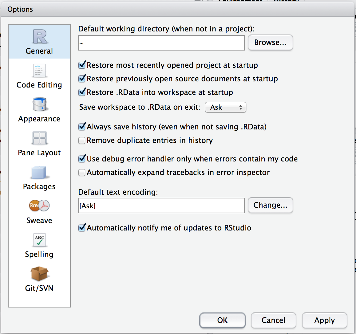
Figure 2.6: The options window in RStudio. On a Mac, you can open this window by going to the “RStudio” menu and selecting “Preferences.” On a Windows machine you go to the “Tools” menu and select “Global Options”
2.14 Summary
Every book that tries to introduce basic programming ideas to novices has to cover roughly the same topics, and in roughly the same order. Mine is no exception, and so in the grand tradition of doing it just the same way everyone else did it, this chapter covered the following topics:
- Getting started. We downloaded and installed R and RStudio
- Basic commands. We talked a bit about the logic of how R works and in particular how to type commands into the R console (Section @ref(#firstcommand), and in doing so learned how to perform basic calculations using the arithmetic operators
+,-,*,/and^. - Introduction to functions. We saw several different functions, three that are used to perform numeric calculations (
sqrt(),abs(),round(), one that applies to text (nchar(); Section 2.10.1), and one that works on any variable (length(); Section 2.9.5). In doing so, we talked a bit about how argument names work, and learned about default values for arguments. (Section 2.7.1) - Introduction to variables. We learned the basic idea behind variables, and how to assign values to variables using the assignment operator
<-(Section 2.6). We also learned how to create vectors using the combine functionc()(Section 2.9). - Data types. Learned the distinction between numeric, character and logical data; including the basics of how to enter and use each of them. (Sections 2.6 to 2.11)
- Logical operations. Learned how to use the logical operators
==,!=,<,>,<=,=>,!,&and|. And learned how to use logical indexing. (Section 2.12)
We still haven’t arrived at anything that resembles a “data set,” of course. Maybe the next Chapter will get us a bit closer…
2.15 Additional R concepts
Form follows function
– Louis Sullivan
So far, our main goal was to get started in R. As we go through the book we’ll run into a lot of new R concepts, which I’ll explain alongside the relevant data analysis concepts. However, there’s still quite a few things that I need to talk about now, otherwise we’ll run into problems when we start trying to work with data and do statistics. So that’s the goal in this section: to build on the introductory content from the last section, to get you to the point that we can start using R for statistics. Broadly speaking, the section comes in two parts. The first half of the section is devoted to the “mechanics” of R: installing and loading packages, managing the workspace, navigating the file system, and loading and saving data. In the second half, I’ll talk more about what kinds of variables exist in R, and introduce three new kinds of variables: factors, data frames and formulas. I’ll finish up by talking a little bit about the help documentation in R as well as some other avenues for finding assistance. In general, I’m not trying to be comprehensive in this chapter, I’m trying to make sure that you’ve got the basic foundations needed to tackle the content that comes later in the book. However, a lot of the topics are revisited in more detail later, especially in Chapters ?? and ??.
2.17 Installing and loading packages
In this section I discuss R packages, since almost all of the functions you might want to use in R come in packages. A package is basically just a big collection of functions, data sets and other R objects that are all grouped together under a common name. Some packages are already installed when you put R on your computer, but the vast majority of them of R packages are out there on the internet, waiting for you to download, install and use them.
When I first started writing this book, RStudio didn’t really exist as a viable option for using R, and as a consequence I wrote a very lengthy section that explained how to do package management using raw R commands. It’s not actually terribly hard to work with packages that way, but it’s clunky and unpleasant. Fortunately, we don’t have to do things that way anymore. In this section, I’ll describe how to work with packages using the RStudio tools, because they’re so much simpler. Along the way, you’ll see that whenever you get RStudio to do something (e.g., install a package), you’ll actually see the R commands that get created. I’ll explain them as we go, because I think that helps you understand what’s going on.
However, before we get started, there’s a critical distinction that you need to understand, which is the difference between having a package installed on your computer, and having a package loaded in R. As of this writing, there are just over 5000 R packages freely available “out there” on the internet.35 When you install R on your computer, you don’t get all of them: only about 30 or so come bundled with the basic R installation. So right now there are about 30 packages “installed” on your computer, and another 5000 or so that are not installed. So that’s what installed means: it means “it’s on your computer somewhere.” The critical thing to remember is that just because something is on your computer doesn’t mean R can use it. In order for R to be able to use one of your 30 or so installed packages, that package must also be “loaded.” Generally, when you open up R, only a few of these packages (about 7 or 8) are actually loaded. Basically what it boils down to is this:
A package must be installed before it can be loaded.
A package must be loaded before it can be used.
This two step process might seem a little odd at first, but the designers of R had very good reasons to do it this way,36 and you get the hang of it pretty quickly.
2.17.1 The package panel in RStudio
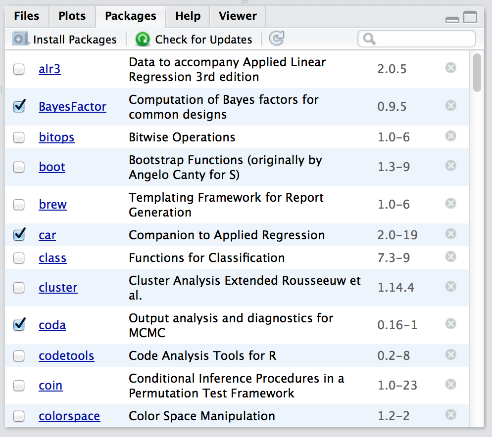
Figure 2.7: The packages panel.
Right, lets get started. The first thing you need to do is look in the lower right hand panel in RStudio. You’ll see a tab labelled “Packages.” Click on the tab, and you’ll see a list of packages that looks something like Figure 2.7. Every row in the panel corresponds to a different package, and every column is a useful piece of information about that package.37 Going from left to right, here’s what each column is telling you:
- The check box on the far left column indicates whether or not the package is loaded.
- The one word of text immediately to the right of the check box is the name of the package.
- The short passage of text next to the name is a brief description of the package.
- The number next to the description tells you what version of the package you have installed.
- The little x-mark next to the version number is a button that you can push to uninstall the package from your computer (you almost never need this).
2.17.2 Loading a package
That seems straightforward enough, so let’s try loading and unloading packades. For this example, I’ll use the foreign package. The foreign package is a collection of tools that are very handy when R needs to interact with files that are produced by other software packages (e.g., SPSS). It comes bundled with R, so it’s one of the ones that you have installed already, but it won’t be one of the ones loaded. Inside the foreign package is a function called read.spss(). It’s a handy little function that you can use to import an SPSS data file into R, so let’s pretend we want to use it. Currently, the foreign package isn’t loaded, so if I ask R to tell me if it knows about a function called read.spss() it tells me that there’s no such thing…
exists( "read.spss" )## [1] FALSENow let’s load the package. In RStudio, the process is dead simple: go to the package tab, find the entry for the foreign package, and check the box on the left hand side. The moment that you do this, you’ll see a command like this appear in the R console:
library("foreign", lib.loc="/Library/Frameworks/R.framework/Versions/3.0/Resources/library")The lib.loc bit will look slightly different on Macs versus on Windows, because that part of the command is just RStudio telling R where to look to find the installed packages. What I’ve shown you above is the Mac version. On a Windows machine, you’ll probably see something that looks like this:
library("foreign", lib.loc="C:/Program Files/R/R-3.0.2/library")But actually it doesn’t matter much. The lib.loc bit is almost always unnecessary. Unless you’ve taken to installing packages in idiosyncratic places (which is something that you can do if you really want) R already knows where to look. So in the vast majority of cases, the command to load the foreign package is just this:
library("foreign")Throughout this book, you’ll often see me typing in library() commands. You don’t actually have to type them in yourself: you can use the RStudio package panel to do all your package loading for you. The only reason I include the library() commands sometimes is as a reminder to you to make sure that you have the relevant package loaded. Oh, and I suppose we should check to see if our attempt to load the package actually worked. Let’s see if R now knows about the existence of the read.spss() function…
exists( "read.spss" )## [1] TRUEYep. All good.
2.17.3 Unloading a package
Sometimes, especially after a long session of working with R, you find yourself wanting to get rid of some of those packages that you’ve loaded. The RStudio package panel makes this exactly as easy as loading the package in the first place. Find the entry corresponding to the package you want to unload, and uncheck the box. When you do that for the foreign package, you’ll see this command appear on screen:
detach("package:foreign", unload=TRUE)And the package is unloaded. We can verify this by seeing if the read.spss() function still exists():
exists( "read.spss" )## [1] FALSENope. Definitely gone.
2.17.4 A few extra comments
Sections 2.17.2 and 2.17.3 cover the main things you need to know about loading and unloading packages. However, there’s a couple of other details that I want to draw your attention to. A concrete example is the best way to illustrate. One of the other packages that you already have installed on your computer is the Matrix package, so let’s load that one and see what happens:
library( Matrix )

## Loading required package: lattice
This is slightly more complex than the output that we got last time, but it’s not too complicated. The Matrix package makes use of some of the tools in the lattice package, and R has kept track of this dependency. So when you try to load the Matrix package, R recognises that you’re also going to need to have the lattice package loaded too. As a consequence, both packages get loaded, and R prints out a helpful little note on screen to tell you that it’s done so.
R is pretty aggressive about enforcing these dependencies. Suppose, for example, I try to unload the lattice package while the Matrix package is still loaded. This is easy enough to try: all I have to do is uncheck the box next to “lattice” in the packages panel. But if I try this, here’s what happens:
detach("package:lattice", unload=TRUE)

## Error: package `lattice' is required by `Matrix' so will not be detached
R refuses to do it. This can be quite useful, since it stops you from accidentally removing something that you still need. So, if I want to remove both Matrix and lattice, I need to do it in the correct order
Something else you should be aware of. Sometimes you’ll attempt to load a package, and R will print out a message on screen telling you that something or other has been “masked.” This will be confusing to you if I don’t explain it now, and it actually ties very closely to the whole reason why R forces you to load packages separately from installing them. Here’s an example. Two of the package that I’ll refer to a lot in this book are called car and psych. The car package is short for “Companion to Applied Regression” (which is a really great book, I’ll add), and it has a lot of tools that I’m quite fond of. The car package was written by a guy called John Fox, who has written a lot of great statistical tools for social science applications. The psych package was written by William Revelle, and it has a lot of functions that are very useful for psychologists in particular, especially in regards to psychometric techniques. For the most part, car and psych are quite unrelated to each other. They do different things, so not surprisingly almost all of the function names are different. But… there’s one exception to that. The car package and the psych package both contain a function called logit().38 This creates a naming conflict. If I load both packages into R, an ambiguity is created. If the user types in logit(100), should R use the logit() function in the car package, or the one in the psych package? The answer is: R uses whichever package you loaded most recently, and it tells you this very explicitly. Here’s what happens when I load the car package, and then afterwards load the psych package:
library(car)## Loading required package: carDatalibrary(psych)##
## Attaching package: 'psych'## The following object is masked from 'package:car':
##
## logitThe output here is telling you that the logit object (i.e., function) in the car package is no longer accessible to you. It’s been hidden (or “masked”) from you by the one in the psych package.39
2.17.5 Downloading new packages
One of the main selling points for R is that there are thousands of packages that have been written for it, and these are all available online. So whereabouts online are these packages to be found, and how do we download and install them? There is a big repository of packages called the “Comprehensive R Archive Network” (CRAN), and the easiest way of getting and installing a new package is from one of the many CRAN mirror sites. Conveniently for us, R provides a function called install.packages() that you can use to do this. Even more conveniently, the RStudio team runs its own CRAN mirror and RStudio has a clean interface that lets you install packages without having to learn how to use the install.packages() command40
Using the RStudio tools is, again, dead simple. In the top left hand corner of the packages panel (Figure 2.7) you’ll see a button called “Install Packages.” If you click on that, it will bring up a window like the one shown in Figure 2.8.
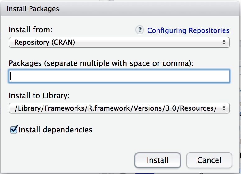
Figure 2.8: The package installation dialog box in RStudio
There are a few different buttons and boxes you can play with. Ignore most of them. Just go to the line that says “Packages” and start typing the name of the package that you want. As you type, you’ll see a dropdown menu appear (Figure 2.9), listing names of packages that start with the letters that you’ve typed so far.
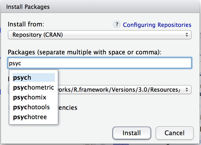
Figure 2.9: When you start typing, you’ll see a dropdown menu suggest a list of possible packages that you might want to install
You can select from this list, or just keep typing. Either way, once you’ve got the package name that you want, click on the install button at the bottom of the window. When you do, you’ll see the following command appear in the R console:
install.packages("psych")This is the R command that does all the work. R then goes off to the internet, has a conversation with CRAN, downloads some stuff, and installs it on your computer. You probably don’t care about all the details of R’s little adventure on the web, but the install.packages() function is rather chatty, so it reports a bunch of gibberish that you really aren’t all that interested in:
trying URL 'http://cran.rstudio.com/bin/macosx/contrib/3.0/psych_1.4.1.tgz'
Content type 'application/x-gzip' length 2737873 bytes (2.6 Mb)
opened URL
==================================================
downloaded 2.6 Mb


The downloaded binary packages are in
    /var/folders/cl/thhsyrz53g73q0w1kb5z3l_80000gn/T//RtmpmQ9VT3/downloaded_packages
Despite the long and tedious response, all thar really means is “I’ve installed the psych package.” I find it best to humour the talkative little automaton. I don’t actually read any of this garbage, I just politely say “thanks” and go back to whatever I was doing.
2.17.6 Updating R and R packages
Every now and then the authors of packages release updated versions. The updated versions often add new functionality, fix bugs, and so on. It’s generally a good idea to update your packages periodically. There’s an update.packages() function that you can use to do this, but it’s probably easier to stick with the RStudio tool. In the packages panel, click on the “Update Packages” button. This will bring up a window that looks like the one shown in Figure 2.10. In this window, each row refers to a package that needs to be updated. You can to tell R which updates you want to install by checking the boxes on the left. If you’re feeling lazy and just want to update everything, click the “Select All” button, and then click the “Install Updates” button. R then prints out a lot of garbage on the screen, individually downloading and installing all the new packages. This might take a while to complete depending on how good your internet connection is. Go make a cup of coffee. Come back, and all will be well.
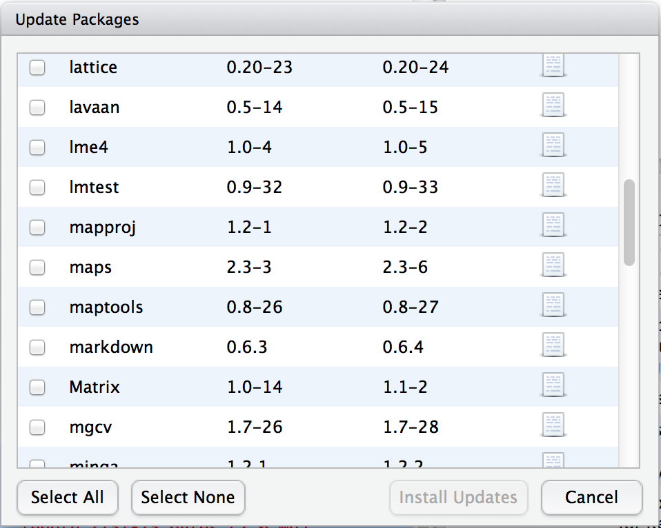
Figure 2.10: The RStudio dialog box for updating packages
About every six months or so, a new version of R is released. You can’t update R from within RStudio (not to my knowledge, at least): to get the new version you can go to the CRAN website and download the most recent version of R, and install it in the same way you did when you originally installed R on your computer. This used to be a slightly frustrating event, because whenever you downloaded the new version of R, you would lose all the packages that you’d downloaded and installed, and would have to repeat the process of re-installing them. This was pretty annoying, and there were some neat tricks you could use to get around this. However, newer versions of R don’t have this problem so I no longer bother explaining the workarounds for that issue.
2.17.7 What packages does this book use?
There are several packages that I make use of in this book. The most prominent ones are:
lsr. This is the Learning Statistics with R package that accompanies this book. It doesn’t have a lot of interesting high-powered tools: it’s just a small collection of handy little things that I think can be useful to novice users. As you get more comfortable with R this package should start to feel pretty useless to you.psych. This package, written by William Revelle, includes a lot of tools that are of particular use to psychologists. In particular, there’s several functions that are particularly convenient for producing analyses or summaries that are very common in psych, but less common in other disciplines.car. This is the Companion to Applied Regression package, which accompanies the excellent book of the same name by (Fox and Weisberg 2011). It provides a lot of very powerful tools, only some of which we’ll touch in this book.
Besides these three, there are a number of packages that I use in a more limited fashion: gplots, sciplot, foreign, effects, R.matlab, gdata, lmtest, and probably one or two others that I’ve missed. There are also a number of packages that I refer to but don’t actually use in this book, such as reshape, compute.es, HistData and multcomp among others. Finally, there are a number of packages that provide more advanced tools that I hope to talk about in future versions of the book, such as sem, ez, nlme and lme4. In any case, whenever I’m using a function that isn’t in the core packages, I’ll make sure to note this in the text.
2.18 Managing the workspace
Let’s suppose that you’re reading through this book, and what you’re doing is sitting down with it once a week and working through a whole chapter in each sitting. Not only that, you’ve been following my advice and typing in all these commands into R. So far during this chapter, you’d have typed quite a few commands, although the only ones that actually involved creating variables were the ones you typed during Section 2.16. As a result, you currently have three variables; seeker, lover, and keeper. These three variables are the contents of your workspace, also referred to as the global environment. The workspace is a key concept in R, so in this section we’ll talk a lot about what it is and how to manage its contents.
2.18.1 Listing the contents of the workspace
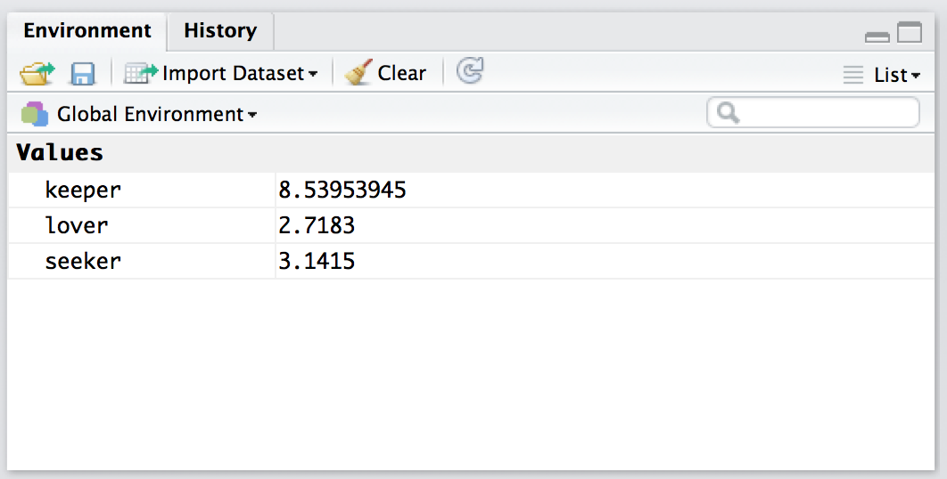
Figure 2.11: The RStudio Environment panel shows you the contents of the workspace. The view shown above is the list view. To switch to the grid view, click on the menu item on the top right that currently reads list. Select grid from the dropdown menu, and then it will switch to a view like the one shown in the other workspace figure
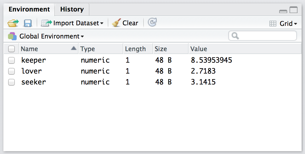
Figure 2.12: The RStudio “Environment” panel shows you the contents of the workspace. Compare this “grid” view to the “list” earlier
The first thing that you need to know how to do is examine the contents of the workspace. If you’re using RStudio, you will probably find that the easiest way to do this is to use the “Environment” panel in the top right hand corner. Click on that, and you’ll see a list that looks very much like the one shown in Figures 2.11 and 2.12. If you’re using the commmand line, then the objects() function may come in handy:
objects()## [1] "any.sales.this.month" "berkeley" "berkeley.small"
## [4] "coef" "days.per.month" "february.sales"
## [7] "greeting" "is.the.Party.correct" "keeper"
## [10] "lover" "months" "profit"
## [13] "projecthome" "revenue" "royalty"
## [16] "sales" "sales.by.month" "seeker"
## [19] "simpson" "stock.levels" "x"
## [22] "xlu"Of course, in the true R tradition, the objects() function has a lot of fancy capabilities that I’m glossing over in this example. Moreover there are also several other functions that you can use, including ls() which is pretty much identical to objects(), and ls.str() which you can use to get a fairly detailed description of all the variables in the workspace. In fact, the lsr package actually includes its own function that you can use for this purpose, called who(). The reason for using the who() function is pretty straightforward: in my everyday work I find that the output produced by the objects() command isn’t quite informative enough, because the only thing it prints out is the name of each variable; but the ls.str() function is too informative, because it prints out a lot of additional information that I really don’t like to look at. The who() function is a compromise between the two. First, now that we’ve got the lsr package installed, we need to load it:
library(lsr)and now we can use the who() function:
who()## -- Name -- -- Class -- -- Size --
## any.sales.this.month logical 12
## berkeley data.frame 39 x 3
## berkeley.small data.frame 46 x 2
## coef numeric 2
## days.per.month numeric 12
## february.sales numeric 1
## greeting character 1
## is.the.Party.correct logical 1
## keeper numeric 1
## lover numeric 1
## months character 12
## profit numeric 12
## projecthome character 1
## revenue numeric 1
## royalty numeric 1
## sales numeric 1
## sales.by.month numeric 12
## seeker numeric 1
## simpson matrix 6 x 5
## stock.levels character 12
## x logical 3
## xlu numeric 1As you can see, the who() function lists all the variables and provides some basic information about what kind of variable each one is and how many elements it contains. Personally, I find this output much easier more useful than the very compact output of the objects() function, but less overwhelming than the extremely verbose ls.str() function. Throughout this book you’ll see me using the who() function a lot. You don’t have to use it yourself: in fact, I suspect you’ll find it easier to look at the RStudio environment panel. But for the purposes of writing a textbook I found it handy to have a nice text based description: otherwise there would be about another 100 or so screenshots added to the book.41
2.18.2 Removing variables from the workspace
Looking over that list of variables, it occurs to me that I really don’t need them any more. I created them originally just to make a point, but they don’t serve any useful purpose anymore, and now I want to get rid of them. I’ll show you how to do this, but first I want to warn you – there’s no “undo” option for variable removal. Once a variable is removed, it’s gone forever unless you save it to disk. I’ll show you how to do that in Section 2.20, but quite clearly we have no need for these variables at all, so we can safely get rid of them.
In RStudio, the easiest way to remove variables is to use the environment panel. Assuming that you’re in grid view (i.e., Figure 2.12), check the boxes next to the variables that you want to delete, then click on the “Clear” button at the top of the panel. When you do this, RStudio will show a dialog box asking you to confirm that you really do want to delete the variables. It’s always worth checking that you really do, because as RStudio is at pains to point out, you can’t undo this. Once a variable is deleted, it’s gone.42 In any case, if you click “yes,” that variable will disappear from the workspace: it will no longer appear in the environment panel, and it won’t show up when you use the who() command.
Suppose you don’t access to RStudio, and you still want to remove variables. This is where the remove function rm() comes in handy. The simplest way to use rm() is just to type in a (comma separated) list of all the variables you want to remove. Let’s say I want to get rid of seeker and lover, but I would like to keep keeper. To do this, all I have to do is type:
rm( seeker, lover )There’s no visible output, but if I now inspect the workspace
who()## -- Name -- -- Class -- -- Size --
## any.sales.this.month logical 12
## berkeley data.frame 39 x 3
## berkeley.small data.frame 46 x 2
## coef numeric 2
## days.per.month numeric 12
## february.sales numeric 1
## greeting character 1
## is.the.Party.correct logical 1
## keeper numeric 1
## months character 12
## profit numeric 12
## projecthome character 1
## revenue numeric 1
## royalty numeric 1
## sales numeric 1
## sales.by.month numeric 12
## simpson matrix 6 x 5
## stock.levels character 12
## x logical 3
## xlu numeric 1I see that there’s only the keeper variable left. As you can see, rm() can be very handy for keeping the workspace tidy.
2.19 Navigating the file system
In this section I talk a little about how R interacts with the file system on your computer. It’s not a terribly interesting topic, but it’s useful. As background to this discussion, I’ll talk a bit about how file system locations work in Section 2.19.1. Once upon a time everyone who used computers could safely be assumed to understand how the file system worked, because it was impossible to successfully use a computer if you didn’t! However, modern operating systems are much more “user friendly,” and as a consequence of this they go to great lengths to hide the file system from users. So these days it’s not at all uncommon for people to have used computers most of their life and not be familiar with the way that computers organise files. If you already know this stuff, skip straight to Section 2.19.2. Otherwise, read on. I’ll try to give a brief introduction that will be useful for those of you who have never been forced to learn how to navigate around a computer using a DOS or UNIX shell.
2.19.1 The file system itself
In this section I describe the basic idea behind file locations and file paths. Regardless of whether you’re using Window, Mac OS or Linux, every file on the computer is assigned a (fairly) human readable address, and every address has the same basic structure: it describes a path that starts from a root location , through as series of folders (or if you’re an old-school computer user, directories), and finally ends up at the file.
On a Windows computer the root is the physical drive43 on which the file is stored, and for most home computers the name of the hard drive that stores all your files is C: and therefore most file names on Windows begin with C:. After that comes the folders, and on Windows the folder names are separated by a \ symbol. So, the complete path to this book on my Windows computer might be something like this:
C:\Users\danRbook\LSR.pdfand what that means is that the book is called LSR.pdf, and it’s in a folder called book which itself is in a folder called dan which itself is … well, you get the idea. On Linux, Unix and Mac OS systems, the addresses look a little different, but they’re more or less identical in spirit. Instead of using the backslash, folders are separated using a forward slash, and unlike Windows, they don’t treat the physical drive as being the root of the file system. So, the path to this book on my Mac might be something like this:
/Users/dan/Rbook/LSR.pdfSo that’s what we mean by the “path” to a file. The next concept to grasp is the idea of a working directory and how to change it. For those of you who have used command line interfaces previously, this should be obvious already. But if not, here’s what I mean. The working directory is just “whatever folder I’m currently looking at.” Suppose that I’m currently looking for files in Explorer (if you’re using Windows) or using Finder (on a Mac). The folder I currently have open is my user directory (i.e., C:\Users\dan or /Users/dan). That’s my current working directory.
The fact that we can imagine that the program is “in” a particular directory means that we can talk about moving from our current location to a new one. What that means is that we might want to specify a new location in relation to our current location. To do so, we need to introduce two new conventions. Regardless of what operating system you’re using, we use . to refer to the current working directory, and .. to refer to the directory above it. This allows us to specify a path to a new location in relation to our current location, as the following examples illustrate. Let’s assume that I’m using my Windows computer, and my working directory is C:\Users\danRbook). The table below shows several addresses in relation to my current one:
| absolute path (i.e., from root) | relative path (i.e. from C:) |
|---|---|
| C:\Users\dan | .. |
| C:\Users | ..\.. \ |
| C:\Users\danRbook\source | .\source |
| C:\Users\dan\nerdstuff | ..\nerdstuff |
There’s one last thing I want to call attention to: the ~ directory. I normally wouldn’t bother, but R makes reference to this concept sometimes. It’s quite common on computers that have multiple users to define ~ to be the user’s home directory. On my Mac, for instance, the home directory ~ for the “dan” user is \Users\dan\. And so, not surprisingly, it is possible to define other directories in terms of their relationship to the home directory. For example, an alternative way to describe the location of the LSR.pdf file on my Mac would be
~Rbook\LSR.pdfThat’s about all you really need to know about file paths. And since this section already feels too long, it’s time to look at how to navigate the file system in R.
2.19.3 Why do the Windows paths use the wrong slash?
Let’s suppose I’m on Windows. As before, I can find out what my current working directory is like this:
getwd()
## [1] "C:/Users/dan/
This seems about right, but you might be wondering why R is displaying a Windows path using the wrong type of slash. The answer is slightly complicated, and has to do with the fact that R treats the \ character as “special” (see Section ??). If you’re deeply wedded to the idea of specifying a path using the Windows style slashes, then what you need to do is to type / whenever you mean \. In other words, if you want to specify the working directory on a Windows computer, you need to use one of the following commands:
setwd( "C:/Users/dan" )
setwd( "C:\\Users\\dan" )
It’s kind of annoying to have to do it this way, but as you’ll see later on in Section ?? it’s a necessary evil. Fortunately, as we’ll see in the next section, RStudio provides a much simpler way of changing directories…
2.19.4 Navigating the file system using the RStudio file panel
Although I think it’s important to understand how all this command line stuff works, in many (maybe even most) situations there’s an easier way. For our purposes, the easiest way to navigate the file system is to make use of RStudio’s built in tools. The “file” panel – the lower right hand area in Figure 2.13 – is actually a pretty decent file browser. Not only can you just point and click on the names to move around the file system, you can also use it to set the working directory, and even load files.
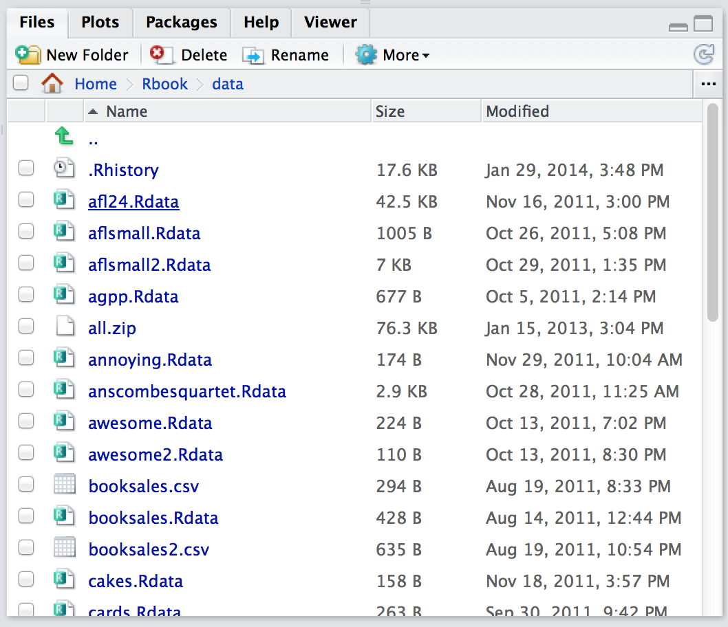
Figure 2.13: The “file panel” is the area shown in the lower right hand corner. It provides a very easy way to browse and navigate your computer using R. See main text for details.
Here’s what you need to do to change the working directory using the file panel. Let’s say I’m looking at the actual screen shown in Figure 2.13. At the top of the file panel you see some text that says “Home \(>\) Rbook \(>\) data.” What that means is that it’s displaying the files that are stored in the
/Users/dan/Rbook/datadirectory on my computer. It does not mean that this is the R working directory. If you want to change the R working directory, using the file panel, you need to click on the button that reads “More.” This will bring up a little menu, and one of the options will be “Set as Working Directory.” If you select that option, then R really will change the working directory. You can tell that it has done so because this command appears in the console:
setwd("~/Rbook/data")In other words, RStudio sends a command to the R console, exactly as if you’d typed it yourself. The file panel can be used to do other things too. If you want to move “up” to the parent folder (e.g., from /Users/dan/Rbook/data to /Users/dan/Rbook click on the “..” link in the file panel. To move to a subfolder, click on the name of the folder that you want to open. You can open some types of file by clicking on them. You can delete files from your computer using the “delete” button, rename them with the “rename” button, and so on.
As you can tell, the file panel is a very handy little tool for navigating the file system. But it can do more than just navigate. As we’ll see later, it can be used to open files. And if you look at the buttons and menu options that it presents, you can even use it to rename, delete, copy or move files, and create new folders. However, since most of that functionality isn’t critical to the basic goals of this book, I’ll let you discover those on your own.
2.20 Loading and saving data
There are several different types of files that are likely to be relevant to us when doing data analysis. There are three in particular that are especially important from the perspective of this book:
- Workspace files are those with a .Rdata file extension. This is the standard kind of file that R uses to store data and variables. They’re called “workspace files” because you can use them to save your whole workspace.
- Comma separated value (CSV) files are those with a .csv file extension. These are just regular old text files, and they can be opened with almost any software. It’s quite typical for people to store data in CSV files, precisely because they’re so simple.
- Script files are those with a .R file extension. These aren’t data files at all; rather, they’re used to save a collection of commands that you want R to execute later. They’re just text files, but we won’t make use of them until Chapter ??.
There are also several other types of file that R makes use of,45 but they’re not really all that central to our interests. There are also several other kinds of data file that you might want to import into R. For instance, you might want to open Microsoft Excel spreadsheets (.xlsx files), or data files that have been saved in the native file formats for other statistics software, such as SPSS, SAS, Minitab, Stata or Systat. Finally, you might have to handle databases. R tries hard to play nicely with other software, so it has tools that let you open and work with any of these and many others. I’ll discuss some of these other possibilities elsewhere in this book (Section ??), but for now I want to focus primarily on the two kinds of data file that you’re most likely to need: .Rdata files and .csv files. In this section I’ll talk about how to load a workspace file, how to import data from a CSV file, and how to save your workspace to a workspace file. Throughout this section I’ll first describe the (sometimes awkward) R commands that do all the work, and then I’ll show you the (much easier) way to do it using RStudio.
2.20.1 Loading workspace files using R
When I used the list.files() command to list the contents of the /Users/dan/Rbook/data directory (in Section 2.19.2), the output referred to a file called booksales.Rdata. Let’s say I want to load the data from this file into my workspace. The way I do this is with the load() function. There are two arguments to this function, but the only one we’re interested in is
file. This should be a character string that specifies a path to the file that needs to be loaded. You can use an absolute path or a relative path to do so.
Using the absolute file path, the command would look like this:
load( file = "/Users/dan/Rbook/data/booksales.Rdata" )but this is pretty lengthy. Given that the working directory (remember, we changed the directory at the end of Section 2.19.4) is /Users/dan/Rbook/data, I could use a relative file path, like so:
load( file = "../data/booksales.Rdata" )However, my preference is usually to change the working directory first, and then load the file. What that would look like is this:
setwd( "../data" )         # move to the data directory
load( "booksales.Rdata" )  # load the data
If I were then to type who() I’d see that there are several new variables in my workspace now. Throughout this book, whenever you see me loading a file, I will assume that the file is actually stored in the working directory, or that you’ve changed the working directory so that R is pointing at the directory that contains the file. Obviously, you don’t need type that command yourself: you can use the RStudio file panel to do the work.
2.20.2 Loading workspace files using RStudio
Okay, so how do we open an .Rdata file using the RStudio file panel? It’s terribly simple. First, use the file panel to find the folder that contains the file you want to load. If you look at Figure 2.13, you can see that there are several .Rdata files listed. Let’s say I want to load the booksales.Rdata file. All I have to do is click on the file name. RStudio brings up a little dialog box asking me to confirm that I do want to load this file. I click yes. The following command then turns up in the console,
load("~/Rbook/data/booksales.Rdata")and the new variables will appear in the workspace (you’ll see them in the Environment panel in RStudio, or if you type who()). So easy it barely warrants having its own section.
2.20.3 Importing data from CSV files using loadingcsv
One quite commonly used data format is the humble “comma separated value” file, also called a CSV file, and usually bearing the file extension .csv. CSV files are just plain old-fashioned text files, and what they store is basically just a table of data. This is illustrated in Figure 2.14, which shows a file called booksales.csv that I’ve created. As you can see, each row corresponds to a variable, and each row represents the book sales data for one month. The first row doesn’t contain actual data though: it has the names of the variables.
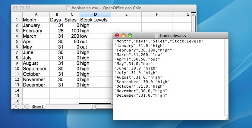
Figure 2.14: The booksales.csv data file. On the left, I’ve opened the file in using a spreadsheet program (OpenOffice), which shows that the file is basically a table. On the right, the same file is open in a standard text editor (the TextEdit program on a Mac), which shows how the file is formatted. The entries in the table are wrapped in quote marks and separated by commas.
If RStudio were not available to you, the easiest way to open this file would be to use the read.csv() function.46 This function is pretty flexible, and I’ll talk a lot more about it’s capabilities in Section ?? for more details, but for now there’s only two arguments to the function that I’ll mention:
file. This should be a character string that specifies a path to the file that needs to be loaded. You can use an absolute path or a relative path to do so.header. This is a logical value indicating whether or not the first row of the file contains variable names. The default value isTRUE.
Therefore, to import the CSV file, the command I need is:
books <- read.csv( file = "booksales.csv" )There are two very important points to notice here. Firstly, notice that I didn’t try to use the load() function, because that function is only meant to be used for .Rdata files. If you try to use load() on other types of data, you get an error. Secondly, notice that when I imported the CSV file I assigned the result to a variable, which I imaginatively called books.47 file. There’s a reason for this. The idea behind an .Rdata file is that it stores a whole workspace. So, if you had the ability to look inside the file yourself you’d see that the data file keeps track of all the variables and their names. So when you load() the file, R restores all those original names. CSV files are treated differently: as far as R is concerned, the CSV only stores one variable, but that variable is big table. So when you import that table into the workspace, R expects you to give it a name.] Let’s have a look at what we’ve got:
print( books )## Month Days Sales Stock.Levels
## 1 January 31 0 high
## 2 February 28 100 high
## 3 March 31 200 low
## 4 April 30 50 out
## 5 May 31 0 out
## 6 June 30 0 high
## 7 July 31 0 high
## 8 August 31 0 high
## 9 September 30 0 high
## 10 October 31 0 high
## 11 November 30 0 high
## 12 December 31 0 highClearly, it’s worked, but the format of this output is a bit unfamiliar. We haven’t seen anything like this before. What you’re looking at is a data frame, which is a very important kind of variable in R, and one I’ll discuss in Section 2.23. For now, let’s just be happy that we imported the data and that it looks about right.
2.20.4 Importing data from CSV files using RStudio
Yet again, it’s easier in RStudio. In the environment panel in RStudio you should see a button called “Import Dataset.” Click on that, and it will give you a couple of options: select the “From Text File…” option, and it will open up a very familiar dialog box asking you to select a file: if you’re on a Mac, it’ll look like the usual Finder window that you use to choose a file; on Windows it looks like an Explorer window. An example of what it looks like on a Mac is shown in Figure 2.15. I’m assuming that you’re familiar with your own computer, so you should have no problem finding the CSV file that you want to import! Find the one you want, then click on the “Open” button. When you do this, you’ll see a window that looks like the one in Figure 2.16.
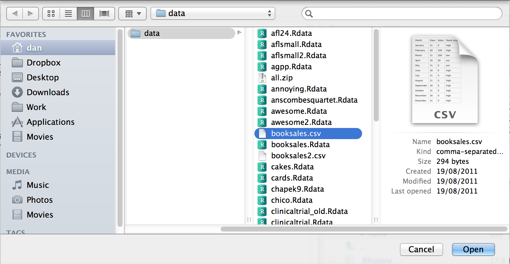
Figure 2.15: A dialog box on a Mac asking you to select the CSV file R should try to import. Mac users will recognise this immediately: it’s the usual way in which a Mac asks you to find a file. Windows users won’t see this: they’ll see the usual explorer window that Windows always gives you when it wants you to select a file.
The import data set window is relatively straightforward to understand.
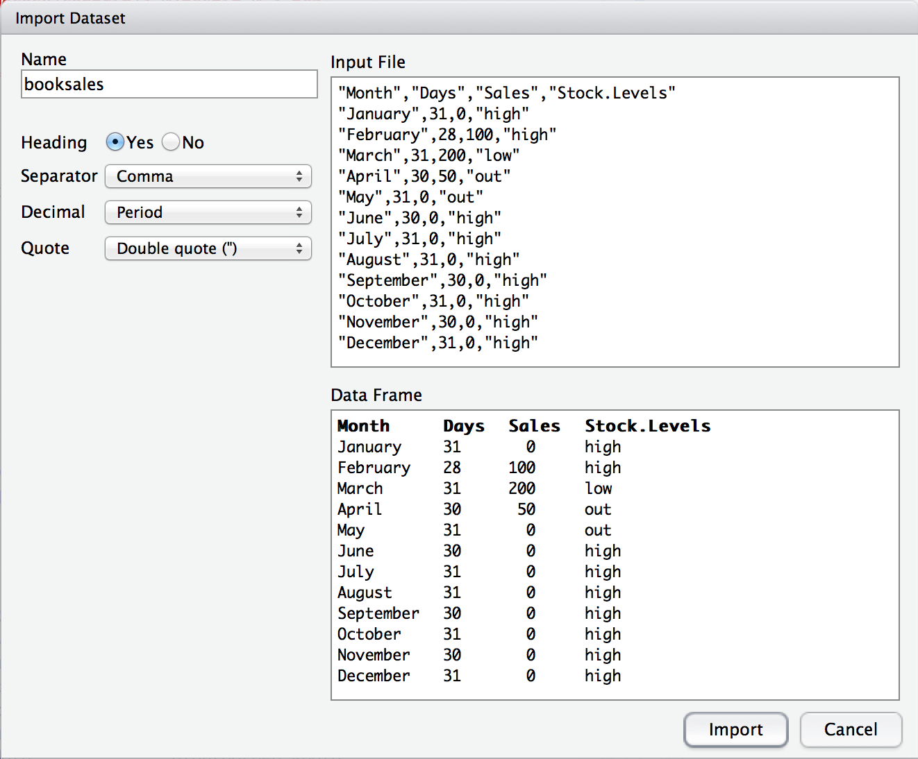
Figure 2.16: The RStudio window for importing a CSV file into R
In the top left corner, you need to type the name of the variable you R to create. By default, that will be the same as the file name: our file is called booksales.csv, so RStudio suggests the name booksales. If you’re happy with that, leave it alone. If not, type something else. Immediately below this are a few things that you can tweak to make sure that the data gets imported correctly:
- Heading. Does the first row of the file contain raw data, or does it contain headings for each variable? The
booksales.csvfile has a header at the top, so I selected “yes.” - Separator. What character is used to separate different entries? In most CSV files this will be a comma (it is “comma separated” after all). But you can change this if your file is different.
- Decimal. What character is used to specify the decimal point? In English speaking countries, this is almost always a period (i.e.,
.). That’s not universally true: many European countries use a comma. So you can change that if you need to. - Quote. What character is used to denote a block of text? That’s usually going to be a double quote mark. It is for the
booksales.csvfile, so that’s what I selected.
The nice thing about the RStudio window is that it shows you the raw data file at the top of the window, and it shows you a preview of the data at the bottom. If the data at the bottom doesn’t look right, try changing some of the settings on the left hand side. Once you’re happy, click “Import.” When you do, two commands appear in the R console:
booksales <- read.csv("~/Rbook/data/booksales.csv")
View(booksales)
The first of these commands is the one that loads the data. The second one will display a pretty table showing the data in RStudio.
2.20.5 Saving a workspace file using save
Not surprisingly, saving data is very similar to loading data. Although RStudio provides a simple way to save files (see below), it’s worth understanding the actual commands involved. There are two commands you can use to do this, save() and save.image(). If you’re happy to save all of the variables in your workspace into the data file, then you should use save.image(). And if you’re happy for R to save the file into the current working directory, all you have to do is this:
save.image( file = "myfile.Rdata" )Since file is the first argument, you can shorten this to save.image("myfile.Rdata"); and if you want to save to a different directory, then (as always) you need to be more explicit about specifying the path to the file, just as we discussed in Section 2.19. Suppose, however, I have several variables in my workspace, and I only want to save some of them. For instance, I might have this as my workspace:
who()
##   -- Name --   -- Class --   -- Size --
##   data         data.frame    3 x 2
##   handy        character     1
##   junk         numeric       1
I want to save data and handy, but not junk. But I don’t want to delete junk right now, because I want to use it for something else later on. This is where the save() function is useful, since it lets me indicate exactly which variables I want to save. Here is one way I can use the save function to solve my problem:
save(data, handy, file = "myfile.Rdata")Importantly, you must specify the name of the file argument. The reason is that if you don’t do so, R will think that "myfile.Rdata" is actually a variable that you want to save, and you’ll get an error message. Finally, I should mention a second way to specify which variables the save() function should save, which is to use the list argument. You do so like this:
save.me <- c("data", "handy")   # the variables to be saved
save( file = "booksales2.Rdata", list = save.me )   # the command to save them
2.20.6 Saving a workspace file using RStudio
RStudio allows you to save the workspace pretty easily. In the environment panel (Figures 2.11 and 2.12) you can see the “save” button. There’s no text, but it’s the same icon that gets used on every computer everywhere: it’s the one that looks like a floppy disk. You know, those things that haven’t been used in about 20 years. Alternatively, go to the “Session” menu and click on the “Save Workspace As…” option.48 This will bring up the standard “save” dialog box for your operating system (e.g., on a Mac it’ll look a little bit like the loading dialog box in Figure 2.15). Type in the name of the file that you want to save it to, and all the variables in your workspace will be saved to disk. You’ll see an R command like this one
save.image("~/Desktop/Untitled.RData")Pretty straightforward, really.
2.20.7 Other things you might want to save
Until now, we’ve talked mostly about loading and saving data. Other things you might want to save include:
The output. Sometimes you might also want to keep a copy of all your interactions with R, including everything that you typed in and everything that R did in response. There are some functions that you can use to get R to write its output to a file rather than to print onscreen (e.g.,
sink()), but to be honest, if you do want to save the R output, the easiest thing to do is to use the mouse to select the relevant text in the R console, go to the “Edit” menu in RStudio and select “Copy.” The output has now been copied to the clipboard. Now open up your favourite text editor or word processing software, and paste it. And you’re done. However, this will only save the contents of the console, not the plots you’ve drawn (assuming you’ve drawn some). We’ll talk about saving images later on.A script. While it is possible – and sometimes handy – to save the R output as a method for keeping a copy of your statistical analyses, another option that people use a lot (especially when you move beyond simple “toy” analyses) is to write scripts. A script is a text file in which you write out all the commands that you want R to run. You can write your script using whatever software you like. In real world data analysis writing scripts is a key skill – and as you become familiar with R you’ll probably find that most of what you do involves scripting rather than typing commands at the R prompt. However, you won’t need to do much scripting initially, so we’ll leave that until Chapter ??.
2.21 Useful things to know about variables
In Chapter 2 I talked a lot about variables, how they’re assigned and some of the things you can do with them, but there’s a lot of additional complexities. That’s not a surprise of course. However, some of those issues are worth drawing your attention to now. So that’s the goal of this section; to cover a few extra topics. As a consequence, this section is basically a bunch of things that I want to briefly mention, but don’t really fit in anywhere else. In short, I’ll talk about several different issues in this section, which are only loosely connected to one another.
2.21.1 Special values
The first thing I want to mention are some of the “special” values that you might see R produce. Most likely you’ll see them in situations where you were expecting a number, but there are quite a few other ways you can encounter them. These values are Inf, NaN, NA and NULL. These values can crop up in various different places, and so it’s important to understand what they mean.
- Infinity (
Inf). The easiest of the special values to explain isInf, since it corresponds to a value that is infinitely large. You can also have-Inf. The easiest way to getInfis to divide a positive number by 0:
1 / 0## [1] InfIn most real world data analysis situations, if you’re ending up with infinite numbers in your data, then something has gone awry. Hopefully you’ll never have to see them.
- Not a Number (
NaN). The special value ofNaNis short for “not a number,” and it’s basically a reserved keyword that means “there isn’t a mathematically defined number for this.” If you can remember your high school maths, remember that it is conventional to say that \(0/0\) doesn’t have a proper answer: mathematicians would say that \(0/0\) is undefined. R says that it’s not a number:
0 / 0## [1] NaNNevertheless, it’s still treated as a “numeric” value. To oversimplify, NaN corresponds to cases where you asked a proper numerical question that genuinely has no meaningful answer.
Not available (
NA).NAindicates that the value that is “supposed” to be stored here is missing. To understand what this means, it helps to recognise that theNAvalue is something that you’re most likely to see when analysing data from real world experiments. Sometimes you get equipment failures, or you lose some of the data, or whatever. The point is that some of the information that you were “expecting” to get from your study is just plain missing. Note the difference betweenNAandNaN. ForNaN, we really do know what’s supposed to be stored; it’s just that it happens to correspond to something like \(0/0\) that doesn’t make any sense at all. In contrast,NAindicates that we actually don’t know what was supposed to be there. The information is missing.No value (
NULL). TheNULLvalue takes this “absence” concept even further. It basically asserts that the variable genuinely has no value whatsoever. This is quite different to bothNaNandNA. ForNaNwe actually know what the value is, because it’s something insane like \(0/0\). ForNA, we believe that there is supposed to be a value “out there,” but a dog ate our homework and so we don’t quite know what it is. But forNULLwe strongly believe that there is no value at all.
2.21.2 Assigning names to vector elements
One thing that is sometimes a little unsatisfying about the way that R prints out a vector is that the elements come out unlabelled. Here’s what I mean. Suppose I’ve got data reporting the quarterly profits for some company. If I just create a no-frills vector, I have to rely on memory to know which element corresponds to which event. That is:
profit <- c( 3.1, 0.1, -1.4, 1.1 )
profit
## [1] 3.1 0.1 -1.4 1.1You can probably guess that the first element corresponds to the first quarter, the second element to the second quarter, and so on, but that’s only because I’ve told you the back story and because this happens to be a very simple example. In general, it can be quite difficult. This is where it can be helpful to assign names to each of the elements. Here’s how you do it:
names(profit) <- c("Q1","Q2","Q3","Q4")
profit
## Q1 Q2 Q3 Q4
## 3.1 0.1 -1.4 1.1This is a slightly odd looking command, admittedly, but it’s not too difficult to follow. All we’re doing is assigning a vector of labels (character strings) to names(profit). You can always delete the names again by using the command names(profit) <- NULL. It’s also worth noting that you don’t have to do this as a two stage process. You can get the same result with this command:
profit <- c( "Q1" = 3.1, "Q2" = 0.1, "Q3" = -1.4, "Q4" = 1.1 )
profit
## Q1 Q2 Q3 Q4
## 3.1 0.1 -1.4 1.1The important things to notice are that (a) this does make things much easier to read, but (b) the names at the top aren’t the “real” data. The value of profit[1] is still 3.1; all I’ve done is added a name to profit[1] as well. Nevertheless, names aren’t purely cosmetic, since R allows you to pull out particular elements of the vector by referring to their names:
profit["Q1"]## Q1
## 3.1And if I ever need to pull out the names themselves, then I just type names(profit).
2.21.3 Variable classes
As we’ve seen, R allows you to store different kinds of data. In particular, the variables we’ve defined so far have either been character data (text), numeric data, or logical data.49 It’s important that we remember what kind of information each variable stores (and even more important that R remembers) since different kinds of variables allow you to do different things to them. For instance, if your variables have numerical information in them, then it’s okay to multiply them together:
x <- 5   # x is numeric
y <- 4   # y is numeric
x * y
## [1] 20But if they contain character data, multiplication makes no sense whatsoever, and R will complain if you try to do it:
x <- "apples"   # x is character
y <- "oranges"  # y is character
x * y
## Error in x * y: non-numeric argument to binary operatorEven R is smart enough to know you can’t multiply "apples" by "oranges". It knows this because the quote marks are indicators that the variable is supposed to be treated as text, not as a number.
This is quite useful, but notice that it means that R makes a big distinction between 5 and "5". Without quote marks, R treats 5 as the number five, and will allow you to do calculations with it. With the quote marks, R treats "5" as the textual character five, and doesn’t recognise it as a number any more than it recognises "p" or "five" as numbers. As a consequence, there’s a big difference between typing x <- 5 and typing x <- "5". In the former, we’re storing the number 5; in the latter, we’re storing the character "5". Thus, if we try to do multiplication with the character versions, R gets stroppy:
x <- "5"   # x is character
y <- "4"   # y is character
x * y
## Error in x * y: non-numeric argument to binary operatorOkay, let’s suppose that I’ve forgotten what kind of data I stored in the variable x (which happens depressingly often). R provides a function that will let us find out. Or, more precisely, it provides three functions: class(), mode() and typeof(). Why the heck does it provide three functions, you might be wondering? Basically, because R actually keeps track of three different kinds of information about a variable:
- The class of a variable is a “high level” classification, and it captures psychologically (or statistically) meaningful distinctions. For instance
"2011-09-12"and"my birthday"are both text strings, but there’s an important difference between the two: one of them is a date. So it would be nice if we could get R to recognise that"2011-09-12"is a date, and allow us to do things like add or subtract from it. The class of a variable is what R uses to keep track of things like that. Because the class of a variable is critical for determining what R can or can’t do with it, theclass()function is very handy. - The mode of a variable refers to the format of the information that the variable stores. It tells you whether R has stored text data or numeric data, for instance, which is kind of useful, but it only makes these “simple” distinctions. It can be useful to know about, but it’s not the main thing we care about. So I’m not going to use the
mode()function very much.50 - The type of a variable is a very low level classification. We won’t use it in this book, but (for those of you that care about these details) this is where you can see the distinction between integer data, double precision numeric, etc. Almost none of you actually will care about this, so I’m not even going to bother demonstrating the
typeof()function.
For purposes, it’s the class() of the variable that we care most about. Later on, I’ll talk a bit about how you can convince R to “coerce” a variable to change from one class to another (Section ??). That’s a useful skill for real world data analysis, but it’s not something that we need right now. In the meantime, the following examples illustrate the use of the class() function:
x <- "hello world"     # x is text
class(x)
## [1] "character"x <- TRUE # x is logical
class(x)## [1] "logical"x <- 100 # x is a number
class(x)## [1] "numeric"Exciting, no?
2.22 Factors
Okay, it’s time to start introducing some of the data types that are somewhat more specific to statistics. If you remember back to Chapter 1.6, when we assign numbers to possible outcomes, these numbers can mean quite different things depending on what kind of variable we are attempting to measure. In particular, we commonly make the distinction between nominal, ordinal, interval and ratio scale data. How do we capture this distinction in R? Currently, we only seem to have a single numeric data type. That’s probably not going to be enough, is it?
A little thought suggests that the numeric variable class in R is perfectly suited for capturing ratio scale data. For instance, if I were to measure response time (RT) for five different events, I could store the data in R like this:
RT <- c(342, 401, 590, 391, 554)where the data here are measured in milliseconds, as is conventional in the psychological literature. It’s perfectly sensible to talk about “twice the response time,” \(2 \times \mbox{RT}\), or the “response time plus 1 second,” \(\mbox{RT} + 1000\), and so both of the following are perfectly reasonable things for R to do:
2 * RT## [1] 684 802 1180 782 1108RT + 1000## [1] 1342 1401 1590 1391 1554And to a lesser extent, the “numeric” class is okay for interval scale data, as long as we remember that multiplication and division aren’t terribly interesting for these sorts of variables. That is, if my IQ score is 110 and yours is 120, it’s perfectly okay to say that you’re 10 IQ points smarter than me51, but it’s not okay to say that I’m only 92% as smart as you are, because intelligence doesn’t have a natural zero.52 We might even be willing to tolerate the use of numeric variables to represent ordinal scale variables, such as those that you typically get when you ask people to rank order items (e.g., like we do in Australian elections), though as we will see R actually has a built in tool for representing ordinal data (see Section ??) However, when it comes to nominal scale data, it becomes completely unacceptable, because almost all of the “usual” rules for what you’re allowed to do with numbers don’t apply to nominal scale data. It is for this reason that R has factors.
2.22.1 Introducing factors
Suppose, I was doing a study in which people could belong to one of three different treatment conditions. Each group of people were asked to complete the same task, but each group received different instructions. Not surprisingly, I might want to have a variable that keeps track of what group people were in. So I could type in something like this
group <- c(1,1,1,2,2,2,3,3,3)so that group[i] contains the group membership of the i-th person in my study. Clearly, this is numeric data, but equally obviously this is a nominal scale variable. There’s no sense in which “group 1” plus “group 2” equals “group 3,” but nevertheless if I try to do that, R won’t stop me because it doesn’t know any better:
group + 2## [1] 3 3 3 4 4 4 5 5 5Apparently R seems to think that it’s allowed to invent “group 4” and “group 5,” even though they didn’t actually exist. Unfortunately, R is too stupid to know any better: it thinks that 3 is an ordinary number in this context, so it sees no problem in calculating 3 + 2. But since we’re not that stupid, we’d like to stop R from doing this. We can do so by instructing R to treat group as a factor. This is easy to do using the as.factor() function.53
group <- as.factor(group)
group
## [1] 1 1 1 2 2 2 3 3 3
## Levels: 1 2 3It looks more or less the same as before (though it’s not immediately obvious what all that Levels rubbish is about), but if we ask R to tell us what the class of the group variable is now, it’s clear that it has done what we asked:
class(group)## [1] "factor"Neat. Better yet, now that I’ve converted group to a factor, look what happens when I try to add 2 to it:
group + 2## Warning in Ops.factor(group, 2): '+' not meaningful for factors## [1] NA NA NA NA NA NA NA NA NAThis time even R is smart enough to know that I’m being an idiot, so it tells me off and then produces a vector of missing values. (i.e., NA: see Section 2.21.1).
2.22.2 Labelling the factor levels
I have a confession to make. My memory is not infinite in capacity; and it seems to be getting worse as I get older. So it kind of annoys me when I get data sets where there’s a nominal scale variable called gender, with two levels corresponding to males and females. But when I go to print out the variable I get something like this:
gender## [1] 1 1 1 1 1 2 2 2 2
## Levels: 1 2Okaaaay. That’s not helpful at all, and it makes me very sad. Which number corresponds to the males and which one corresponds to the females? Wouldn’t it be nice if R could actually keep track of this? It’s way too hard to remember which number corresponds to which gender. To fix this problem what we need to do is assign meaningful labels to the different levels of each factor. We can do that like this:
levels(group) <- c("group 1", "group 2", "group 3")
print(group)
## [1] group 1 group 1 group 1 group 2 group 2 group 2 group 3 group 3 group 3
## Levels: group 1 group 2 group 3levels(gender) <- c("male", "female")
print(gender)## [1] male male male male male female female female female
## Levels: male femaleThat’s much easier on the eye.
2.22.3 Moving on…
Factors are very useful things, and we’ll use them a lot in this book: they’re the main way to represent a nominal scale variable. And there are lots of nominal scale variables out there. I’ll talk more about factors in Section ??, but for now you know enough to be able to get started.
2.23 Data frames
It’s now time to go back and deal with the somewhat confusing thing that happened in Section 2.20.3 when we tried to open up a CSV file. Apparently we succeeded in loading the data, but it came to us in a very odd looking format. At the time, I told you that this was a data frame. Now I’d better explain what that means.
2.23.1 Introducing data frames
In order to understand why R has created this funny thing called a data frame, it helps to try to see what problem it solves. So let’s go back to the little scenario that I used when introducing factors in Section 2.22. In that section I recorded the group and gender for all 9 participants in my study. Let’s also suppose I recorded their ages and their score on “Dan’s Terribly Exciting Psychological Test”:
age <- c(17, 19, 21, 37, 18, 19, 47, 18, 19)
score <- c(12, 10, 11, 15, 16, 14, 25, 21, 29)
Assuming no other variables are in the workspace, if I type who() I get this:
who()## -- Name -- -- Class -- -- Size --
## age numeric 9
## any.sales.this.month logical 12
## berkeley data.frame 39 x 3
## berkeley.small data.frame 46 x 2
## coef numeric 2
## days.per.month numeric 12
## february.sales numeric 1
## gender factor 9
## greeting character 1
## group factor 9
## is.the.Party.correct logical 1
## months character 12
## projecthome character 1
## revenue numeric 1
## royalty numeric 1
## sales numeric 1
## sales.by.month numeric 12
## score numeric 9
## simpson matrix 6 x 5
## stock.levels character 12
## xlu numeric 1So there are four variables in the workspace, age, gender, group and score. And it just so happens that all four of them are the same size (i.e., they’re all vectors with 9 elements). Aaaand it just so happens that age[1] corresponds to the age of the first person, and gender[1] is the gender of that very same person, etc. In other words, you and I both know that all four of these variables correspond to the same data set, and all four of them are organised in exactly the same way.
However, R doesn’t know this! As far as it’s concerned, there’s no reason why the age variable has to be the same length as the gender variable; and there’s no particular reason to think that age[1] has any special relationship to gender[1] any more than it has a special relationship to gender[4]. In other words, when we store everything in separate variables like this, R doesn’t know anything about the relationships between things. It doesn’t even really know that these variables actually refer to a proper data set. The data frame fixes this: if we store our variables inside a data frame, we’re telling R to treat these variables as a single, fairly coherent data set.
To see how they do this, let’s create one. So how do we create a data frame? One way we’ve already seen: if we import our data from a CSV file, R will store it as a data frame. A second way is to create it directly from some existing variables using the data.frame() function. All you have to do is type a list of variables that you want to include in the data frame. The output of a data.frame() command is, well, a data frame. So, if I want to store all four variables from my experiment in a data frame called expt I can do so like this:
expt <- data.frame ( age, gender, group, score )
expt
## age gender group score
## 1 17 male group 1 12
## 2 19 male group 1 10
## 3 21 male group 1 11
## 4 37 male group 2 15
## 5 18 male group 2 16
## 6 19 female group 2 14
## 7 47 female group 3 25
## 8 18 female group 3 21
## 9 19 female group 3 29Note that expt is a completely self-contained variable. Once you’ve created it, it no longer depends on the original variables from which it was constructed. That is, if we make changes to the original age variable, it will not lead to any changes to the age data stored in expt.
2.23.2 Pulling out the contents of the data frame using $
At this point, our workspace contains only the one variable, a data frame called expt. But as we can see when we told R to print the variable out, this data frame contains 4 variables, each of which has 9 observations. So how do we get this information out again? After all, there’s no point in storing information if you don’t use it, and there’s no way to use information if you can’t access it. So let’s talk a bit about how to pull information out of a data frame.
The first thing we might want to do is pull out one of our stored variables, let’s say score. One thing you might try to do is ignore the fact that score is locked up inside the expt data frame. For instance, you might try to print it out like this:
score## Error in eval(expr, envir, enclos): object 'score' not foundThis doesn’t work, because R doesn’t go “peeking” inside the data frame unless you explicitly tell it to do so. There’s actually a very good reason for this, which I’ll explain in a moment, but for now let’s just assume R knows what it’s doing. How do we tell R to look inside the data frame? As is always the case with R there are several ways. The simplest way is to use the $ operator to extract the variable you’re interested in, like this:
expt$score## [1] 12 10 11 15 16 14 25 21 292.23.3 Getting information about a data frame
One problem that sometimes comes up in practice is that you forget what you called all your variables. Normally you might try to type objects() or who(), but neither of those commands will tell you what the names are for those variables inside a data frame! One way is to ask R to tell you what the names of all the variables stored in the data frame are, which you can do using the names() function:
names(expt)## [1] "age" "gender" "group" "score"An alternative method is to use the who() function, as long as you tell it to look at the variables inside data frames. If you set expand = TRUE then it will not only list the variables in the workspace, but it will “expand” any data frames that you’ve got in the workspace, so that you can see what they look like. That is:
who(expand = TRUE)## -- Name -- -- Class -- -- Size --
## any.sales.this.month logical 12
## berkeley data.frame 39 x 3
## $women.apply numeric 39
## $total.admit numeric 39
## $number.apply numeric 39
## berkeley.small data.frame 46 x 2
## $women.apply numeric 46
## $total.admit numeric 46
## coef numeric 2
## days.per.month numeric 12
## expt data.frame 9 x 4
## $age numeric 9
## $gender factor 9
## $group factor 9
## $score numeric 9
## february.sales numeric 1
## greeting character 1
## is.the.Party.correct logical 1
## months character 12
## projecthome character 1
## revenue numeric 1
## royalty numeric 1
## sales numeric 1
## sales.by.month numeric 12
## simpson matrix 6 x 5
## stock.levels character 12
## xlu numeric 1or, since expand is the first argument in the who() function you can just type who(TRUE). I’ll do that a lot in this book.
2.23.4 Looking for more on data frames?
There’s a lot more that can be said about data frames: they’re fairly complicated beasts, and the longer you use R the more important it is to make sure you really understand them. We’ll talk a lot more about them in Chapter ??.
2.24 Lists
The next kind of data I want to mention are lists. Lists are an extremely fundamental data structure in R, and as you start making the transition from a novice to a savvy R user you will use lists all the time. I don’t use lists very often in this book – not directly – but most of the advanced data structures in R are built from lists (e.g., data frames are actually a specific type of list). Because lists are so important to how R stores things, it’s useful to have a basic understanding of them. Okay, so what is a list, exactly? Like data frames, lists are just “collections of variables.” However, unlike data frames – which are basically supposed to look like a nice “rectangular” table of data – there are no constraints on what kinds of variables we include, and no requirement that the variables have any particular relationship to one another. In order to understand what this actually means, the best thing to do is create a list, which we can do using the list() function. If I type this as my command:
Dan <- list( age = 34,
            nerd = TRUE,
            parents = c("Joe","Liz")
)
R creates a new list variable called Dan, which is a bundle of three different variables: age, nerd and parents. Notice, that the parents variable is longer than the others. This is perfectly acceptable for a list, but it wouldn’t be for a data frame. If we now print out the variable, you can see the way that R stores the list:
print( Dan )## $age
## [1] 34
##
## $nerd
## [1] TRUE
##
## $parents
## [1] "Joe" "Liz"As you might have guessed from those $ symbols everywhere, the variables are stored in exactly the same way that they are for a data frame (again, this is not surprising: data frames are a type of list). So you will (I hope) be entirely unsurprised and probably quite bored when I tell you that you can extract the variables from the list using the $ operator, like so:
Dan$nerd## [1] TRUEIf you need to add new entries to the list, the easiest way to do so is to again use $, as the following example illustrates. If I type a command like this
Dan$children <- "Alex"then R creates a new entry to the end of the list called children, and assigns it a value of "Alex". If I were now to print() this list out, you’d see a new entry at the bottom of the printout. Finally, it’s actually possible for lists to contain other lists, so it’s quite possible that I would end up using a command like Dan$children$age to find out how old my son is. Or I could try to remember it myself I suppose.
2.25 Formulas
The last kind of variable that I want to introduce before finally being able to start talking about statistics is the formula. Formulas were originally introduced into R as a convenient way to specify a particular type of statistical model (see Chapter 8) but they’re such handy things that they’ve spread. Formulas are now used in a lot of different contexts, so it makes sense to introduce them early.
Stated simply, a formula object is a variable, but it’s a special type of variable that specifies a relationship between other variables. A formula is specified using the “tilde operator” ~. A very simple example of a formula is shown below:54
formula1 <- out ~ pred
formula1
## out ~ predThe precise meaning of this formula depends on exactly what you want to do with it, but in broad terms it means “the out (outcome) variable, analysed in terms of the pred (predictor) variable.” That said, although the simplest and most common form of a formula uses the “one variable on the left, one variable on the right” format, there are others. For instance, the following examples are all reasonably common
formula2 <-  out ~ pred1 + pred2   # more than one variable on the right
formula3 <-  out ~ pred1 * pred2   # different relationship between predictors
formula4 <-  ~ var1 + var2         # a 'one-sided' formula
and there are many more variants besides. Formulas are pretty flexible things, and so different functions will make use of different formats, depending on what the function is intended to do.
2.26 Generic functions
There’s one really important thing that I omitted when I discussed functions earlier on in Section 2.7, and that’s the concept of a generic function. The two most notable examples that you’ll see in the next few chapters are summary() and plot(), although you’ve already seen an example of one working behind the scenes, and that’s the print() function. The thing that makes generics different from the other functions is that their behaviour changes, often quite dramatically, depending on the class() of the input you give it. The easiest way to explain the concept is with an example. With that in mind, lets take a closer look at what the print() function actually does. I’ll do this by creating a formula, and printing it out in a few different ways. First, let’s stick with what we know:
my.formula <- blah ~ blah.blah    # create a variable of class "formula"
print( my.formula )               # print it out using the generic print() function
## blah ~ blah.blahSo far, there’s nothing very surprising here. But there’s actually a lot going on behind the scenes here. When I type print( my.formula ), what actually happens is the print() function checks the class of the my.formula variable. When the function discovers that the variable it’s been given is a formula, it goes looking for a function called print.formula(), and then delegates the whole business of printing out the variable to the print.formula() function.55 For what it’s worth, the name for a “dedicated” function like print.formula() that exists only to be a special case of a generic function like print() is a method, and the name for the process in which the generic function passes off all the hard work onto a method is called method dispatch. You won’t need to understand the details at all for this book, but you do need to know the gist of it; if only because a lot of the functions we’ll use are actually generics. Anyway, to help expose a little more of the workings to you, let’s bypass the print() function entirely and call the formula method directly:
print.formula( my.formula )       # print it out using the print.formula() method

## Appears to be deprecated
There’s no difference in the output at all. But this shouldn’t surprise you because it was actually the print.formula() method that was doing all the hard work in the first place. The print() function itself is a lazy bastard that doesn’t do anything other than select which of the methods is going to do the actual printing.
Okay, fair enough, but you might be wondering what would have happened if print.formula() didn’t exist? That is, what happens if there isn’t a specific method defined for the class of variable that you’re using? In that case, the generic function passes off the hard work to a “default” method, whose name in this case would be print.default(). Let’s see what happens if we bypass the print() formula, and try to print out my.formula using the print.default() function:
print.default( my.formula ) # print it out using the print.default() method## blah ~ blah.blah
## attr(,"class")
## [1] "formula"
## attr(,".Environment")
## <environment: R_GlobalEnv>Hm. You can kind of see that it is trying to print out the same formula, but there’s a bunch of ugly low-level details that have also turned up on screen. This is because the print.default() method doesn’t know anything about formulas, and doesn’t know that it’s supposed to be hiding the obnoxious internal gibberish that R produces sometimes.
At this stage, this is about as much as we need to know about generic functions and their methods. In fact, you can get through the entire book without learning any more about them than this, so it’s probably a good idea to end this discussion here.
2.27 Getting help
The very last topic I want to mention in this chapter is where to go to find help. Obviously, I’ve tried to make this book as helpful as possible, but it’s not even close to being a comprehensive guide, and there’s thousands of things it doesn’t cover. So where should you go for help?
2.27.1 How to read the help documentation
I have somewhat mixed feelings about the help documentation in R. On the plus side, there’s a lot of it, and it’s very thorough. On the minus side, there’s a lot of it, and it’s very thorough. There’s so much help documentation that it sometimes doesn’t help, and most of it is written with an advanced user in mind. Often it feels like most of the help files work on the assumption that the reader already understands everything about R except for the specific topic that it’s providing help for. What that means is that, once you’ve been using R for a long time and are beginning to get a feel for how to use it, the help documentation is awesome. These days, I find myself really liking the help files (most of them anyway). But when I first started using R I found it very dense.
To some extent, there’s not much I can do to help you with this. You just have to work at it yourself; once you’re moving away from being a pure beginner and are becoming a skilled user, you’ll start finding the help documentation more and more helpful. In the meantime, I’ll help as much as I can by trying to explain to you what you’re looking at when you open a help file. To that end, let’s look at the help documentation for the load() function. To do so, I type either of the following:
?load
help("load")
When I do that, R goes looking for the help file for the “load” topic. If it finds one, Rstudio takes it and displays it in the help panel. Alternatively, you can try a fuzzy search for a help topic
??load
help.search("load")load” topic as our example. Firstly, at the very top we see this:
| load {base} | R Documentation |
Reload Saved Datasets
Description
Reload datasets written with the function save.
Usage
load(file, envir = parent.frame(), verbose = FALSE)
In this instance, the usage section is actually pretty readable. It’s telling you that there are two arguments to the load() function: the first one is called file, and the second one is called envir. It’s also telling you that there is a default value for the envir argument; so if the user doesn’t specify what the value of envir should be, then R will assume that envir = parent.frame(). In contrast, the file argument has no default value at all, so the user must specify a value for it. So in one sense, this section is very straightforward.
The problem, of course, is that you don’t know what the parent.frame() function actually does, so it’s hard for you to know what the envir = parent.frame() bit is all about. What you could do is then go look up the help documents for the parent.frame() function (and sometimes that’s actually a good idea), but often you’ll find that the help documents for those functions are just as dense (if not more dense) than the help file that you’re currently reading. As an alternative, my general approach when faced with something like this is to skim over it, see if I can make any sense of it. If so, great. If not, I find that the best thing to do is ignore it. In fact, the first time I read the help file for the load() function, I had no idea what any of the envir related stuff was about. But fortunately I didn’t have to: the default setting here (i.e., envir = parent.frame()) is actually the thing you want in about 99% of cases, so it’s safe to ignore it.
Basically, what I’m trying to say is: don’t let the scary, incomprehensible parts of the help file intimidate you. Especially because there’s often some parts of the help file that will make sense. Of course, I guarantee you that sometimes this strategy will lead you to make mistakes… often embarrassing mistakes. But it’s still better than getting paralysed with fear.
So, let’s continue on. The next part of the help documentation discusses each of the arguments, and what they’re supposed to do:Arguments
file
|
a (readable binary-mode) connection or a character string giving the name of the file to load (when tilde expansion is done). |
envir
|
the environment where the data should be loaded. |
verbose
|
should item names be printed during loading? |
Okay, so what this is telling us is that the file argument needs to be a string (i.e., text data) which tells R the name of the file to load. It also seems to be hinting that there’s other possibilities too (e.g., a “binary mode connection”), and you probably aren’t quite sure what “tilde expansion” means56. But overall, the meaning is pretty clear.
Turning to the envir argument, it’s now a little clearer what the Usage section was babbling about. The envir argument specifies the name of an environment (see Section 4.3 if you’ve forgotten what environments are) into which R should place the variables when it loads the file. Almost always, this is a no-brainer: you want R to load the data into the same damn environment in which you’re invoking the load() command. That is, if you’re typing load() at the R prompt, then you want the data to be loaded into your workspace (i.e., the global environment). But if you’re writing your own function that needs to load some data, you want the data to be loaded inside that function’s private workspace. And in fact, that’s exactly what the parent.frame() thing is all about. It’s telling the load() function to send the data to the same place that the load() command itself was coming from. As it turns out, if we’d just ignored the envir bit we would have been totally safe. Which is nice to know.
Details
load can load R objects saved in the current or any earlier
format. It can read a compressed file (see save)
directly from a file or from a suitable connection (including a call
to url).
A not-open connection will be opened in mode “rb” and closed
after use. Any connection other than a gzfile or
gzcon connection will be wrapped in gzcon
to allow compressed saves to be handled: note that this leaves the
connection in an altered state (in particular, binary-only), and that
it needs to be closed explicitly (it will not be garbage-collected).
Only R objects saved in the current format (used since R 1.4.0) can be read from a connection. If no input is available on a connection a warning will be given, but any input not in the current format will result in a error.
Loading from an earlier version will give a warning about the
‘magic number’: magic numbers 1971:1977 are from R <
0.99.0, and RD[ABX]1 from R 0.99.0 to R 1.3.1. These are all
obsolete, and you are strongly recommended to re-save such files in a
current format.
The verbose argument is mainly intended for debugging. If it
is TRUE, then as objects from the file are loaded, their
names will be printed to the console. If verbose is set to
an integer value greater than one, additional names corresponding to
attributes and other parts of individual objects will also be printed.
Larger values will print names to a greater depth.
Objects can be saved with references to namespaces, usually as part of the environment of a function or formula. Such objects can be loaded even if the namespace is not available: it is replaced by a reference to the global environment with a warning. The warning identifies the first object with such a reference (but there may be more than one).
Then it tells you what the output value of the function is:
Value
A character vector of the names of objects created, invisibly.
This is usually a bit more interesting, but since the load() function is mainly used to load variables into the workspace rather than to return a value, it’s no surprise that this doesn’t do much or say much. Moving on, we sometimes see a few additional sections in the help file, which can be different depending on what the function is:
Warning
Saved R objects are binary files, even those saved with
ascii = TRUE, so ensure that they are transferred without
conversion of end of line markers. load tries to detect such a
conversion and gives an informative error message.
load(<file>) replaces all existing objects with the same names
in the current environment (typically your workspace,
.GlobalEnv) and hence potentially overwrites important data.
It is considerably safer to use envir = to load into a
different environment, or to attach(file) which
load()s into a new entry in the search path.
Note
file can be a UTF-8-encoded filepath that cannot be translated to
the current locale.
Yeah, yeah. Warning, warning, blah blah blah. Towards the bottom of the help file, we see something like this, which suggests a bunch of related topics that you might want to look at. These can be quite helpful:
See Also
save, download.file; further
attach as wrapper for load().
For other interfaces to the underlying serialization format, see
unserialize and readRDS.
load” help file:
Examples
## save all data
xx <- pi # to ensure there is some data
save(list = ls(all = TRUE), file= "all.rda")
rm(xx)

## restore the saved values to the current environment
local({
   load("all.rda")
   ls()
})

xx <- exp(1:3)
## restore the saved values to the user's workspace
load("all.rda") ## which is here *equivalent* to
## load("all.rda", .GlobalEnv)
## This however annihilates all objects in .GlobalEnv with the same names !
xx # no longer exp(1:3)
rm(xx)
attach("all.rda") # safer and will warn about masked objects w/ same name in .GlobalEnv
ls(pos = 2)
##  also typically need to cleanup the search path:
detach("file:all.rda")

## clean up (the example):
unlink("all.rda")


## Not run:
con <- url("http://some.where.net/R/data/example.rda")
## print the value to see what objects were created.
print(load(con))
close(con) # url() always opens the connection

## End(Not run)
As you can see, they’re pretty dense, and not at all obvious to the novice user. However, they do provide good examples of the various different things that you can do with the load() function, so it’s not a bad idea to have a look at them, and to try not to find them too intimidating.
2.27.2 Other resources
- The Rseek website (www.rseek.org). One thing that I really find annoying about the R help documentation is that it’s hard to search properly. When coupled with the fact that the documentation is dense and highly technical, it’s often a better idea to search or ask online for answers to your questions. With that in mind, the Rseek website is great: it’s an R specific search engine. I find it really useful, and it’s almost always my first port of call when I’m looking around.
- The R-help mailing list (see http://www.r-project.org/mail.html for details). This is the official R help mailing list. It can be very helpful, but it’s very important that you do your homework before posting a question. The list gets a lot of traffic. While the people on the list try as hard as they can to answer questions, they do so for free, and you really don’t want to know how much money they could charge on an hourly rate if they wanted to apply market rates. In short, they are doing you a favour, so be polite. Don’t waste their time asking questions that can be easily answered by a quick search on Rseek (it’s rude), make sure your question is clear, and all of the relevant information is included. In short, read the posting guidelines carefully (http://www.r-project.org/posting-guide.html), and make use of the
help.request()function that R provides to check that you’re actually doing what you’re expected.
2.28 Summary
This chapter continued where Chapter 2 left off. The focus was still primarily on introducing basic R concepts, but this time at least you can see how those concepts are related to data analysis:
- Installing, loading and updating packages. Knowing how to extend the functionality of R by installing and using packages is critical to becoming an effective R user
- Getting around. Section 2.18 talked about how to manage your workspace and how to keep it tidy. Similarly, Section 2.19 talked about how to get R to interact with the rest of the file system.
- Loading and saving data. Finally, we encountered actual data files. Loading and saving data is obviously a crucial skill, one we discussed in Section 2.20.
- Useful things to know about variables. In particular, we talked about special values, element names and classes.
- More complex types of variables. R has a number of important variable types that will be useful when analysing real data. I talked about factors in Section 2.22, data frames in Section 2.23, lists in Section 2.24 and formulas in Section 2.25.
- Generic functions. How is it that some function seem to be able to do lots of different things? Section 2.26 tells you how.
- Getting help. Assuming that you’re not looking for counselling, Section 2.27 covers several possibilities. If you are looking for counselling, well, this book really can’t help you there. Sorry.
Taken together, Chapters 2 and 2.15 provide enough of a background that you can finally get started doing some statistics! Yes, there’s a lot more R concepts that you ought to know (and we’ll talk about some of them in Chapters?? and??), but I think that we’ve talked quite enough about programming for the moment. It’s time to see how your experience with programming can be used to do some data analysis…
References
Source: Dismal Light (1968).↩︎
Although R is updated frequently, it doesn’t usually make much of a difference for the sort of work we’ll do in this book. In fact, during the writing of the book I upgraded several times, and didn’t have to change much except these sections describing the downloading.↩︎
If you’re running an older version of the Mac OS, then you need to follow the link to the “old” page (http://cran.r-project.org/bin/macosx/old/). You should be able to find the installer file that you need at the bottom of the page.↩︎
Tip for advanced Mac users. You can run R from the terminal if you want to. The command is just “R.” It behaves like the normal desktop version, except that help documentation behaves like a “man” page instead of opening in a new window.↩︎
This is probably no coincidence: the people who design and distribute the core R language itself are focused on technical stuff. And sometimes they almost seem to forget that there’s an actual human user at the end. The people who design and distribute RStudio are focused on user interface. They want to make R as usable as possible. The two websites reflect that difference.↩︎
Seriously. If you’re in a position to do so, open up R and start typing. The simple act of typing it rather than “just reading” makes a big difference. It makes the concepts more concrete, and it ties the abstract ideas (programming and statistics) to the actual context in which you need to use them. Statistics is something you do, not just something you read about in a textbook.↩︎
If you’re running R from the terminal rather than from RStudio, escape doesn’t work: use CTRL-C instead.↩︎
For advanced users: yes, as you’ve probably guessed, R is printing out the source code for the function.↩︎
If you’re reading this with R open, a good learning trick is to try typing in a few different variations on what I’ve done here. If you experiment with your commands, you’ll quickly learn what works and what doesn’t↩︎
For advanced users: if you want a table showing the complete order of operator precedence in R, type
?Syntax. I haven’t included it in this book since there are quite a few different operators, and we don’t need that much detail. Besides, in practice most people seem to figure it out from seeing examples: until writing this book I never looked at the formal statement of operator precedence for any language I ever coded in, and never ran into any difficulties.↩︎If you are using RStudio, and the “environment” panel (formerly known as the “workspace” panel) is visible when you typed the command, then you probably saw something happening there. That’s to be expected, and is quite helpful. However, there’s two things to note here (1) I haven’t yet explained what that panel does, so for now just ignore it, and (2) this is one of the helpful things RStudio does, not a part of R itself.↩︎
As we’ll discuss later, by doing this we are implicitly using the
print()function↩︎Actually, in keeping with the R tradition of providing you with a billion different screwdrivers (even when you’re actually looking for a hammer) these aren’t the only options. There’s also the
assign()function, and the<<-and->>operators. However, we won’t be using these at all in this book.↩︎A quick reminder: when using operators like
<-and->that span multiple characters, you can’t insert spaces in the middle. That is, if you type- >or< -, R will interpret your command the wrong way. And I will cry.↩︎Actually, you can override any of these rules if you want to, and quite easily. All you have to do is add quote marks or backticks around your non-standard variable name. For instance
`my sales ` <- 350would work just fine, but it’s almost never a good idea to do this.↩︎For very advanced users: there is one exception to this. If you’re naming a function, don’t use
.in the name unless you are intending to make use of the S3 object oriented programming system in R. If you don’t know what S3 is, then you definitely don’t want to be using it! For function naming, there’s been a trend among R users to prefermyFunctionName.↩︎A side note for students with a programming background. Technically speaking, operators are functions in R: the addition operator
+is actually a convenient way of calling the addition function+(). Thus10+20is equivalent to the function call+(20, 30). Not surprisingly, no-one ever uses this version. Because that would be stupid.↩︎A note for the mathematically inclined: R does support complex numbers, but unless you explicitly specify that you want them it assumes all calculations must be real valued. By default, the square root of a negative number is treated as undefined:
sqrt(-9)will produceNaN(not a number) as its output. To get complex numbers, you would typesqrt(-9+0i)and R would now return0+3i. However, since we won’t have any need for complex numbers in this book, I won’t refer to them again.↩︎The two functions discussed previously,
sqrt()andabs(), both only have a single argument,x. So I could have typed something likesqrt(x = 225)orabs(x = -13)earlier. The fact that all these functions usexas the name of the argument that corresponds the “main” variable that you’re working with is no coincidence. That’s a fairly widely used convention. Quite often, the writers of R functions will try to use conventional names like this to make your life easier. Or at least that’s the theory. In practice it doesn’t always work as well as you’d hope.↩︎For advanced users: obviously, this isn’t just an RStudio thing. If you’re running R in a terminal window, tab autocomplete still works, and does so in exactly the way you’d expect. It’s not as visually pretty as the RStudio version, of course, and lacks some of the cooler features that RStudio provides. I don’t bother to document that here: my assumption is that if you are running R in the terminal then you’re already familiar with using tab autocomplete.↩︎
Incidentally, that always works: if you’ve started typing a command and you want to clear it and start again, hit escape.↩︎
Another method is to start typing some text and then hit the Control key and the up arrow together (on Windows or Linux) or the Command key and the up arrow together (on a Mac). This will bring up a window showing all your recent commands that started with the same text as what you’ve currently typed. That can come in quite handy sometimes.↩︎
Notice that I didn’t specify any argument names here. The
c()function is one of those cases where we don’t use names. We just type all the numbers, and R just dumps them all in a single variable.↩︎Though actually there’s no real need to do this, since R has an inbuilt variable called
month.namethat you can use for this purpose.↩︎I offer up my teenage attempts to be “cool” as evidence that some things just can’t be done.↩︎
Note that this is a very different operator to the assignment operator
=that I talked about in Section 2.6. A common typo that people make when trying to write logical commands in R (or other languages, since the “=versus==” distinction is important in most programming languages) is to accidentally type=when you really mean==. Be especially cautious with this – I’ve been programming in various languages since I was a teenager, and I still screw this up a lot. Hm. I think I see why I wasn’t cool as a teenager. And why I’m still not cool.↩︎A note for those of you who have taken a computer science class: yes, R does have a function for exclusive-or, namely
xor(). Also worth noting is the fact that R makes the distinction between element-wise operators&and|and operators that look only at the first element of the vector, namely&&and||. To see the distinction, compare the behaviour of a command likec(FALSE,TRUE) & c(TRUE,TRUE)to the behaviour of something likec(FALSE,TRUE) && c(TRUE,TRUE). If this doesn’t mean anything to you, ignore this footnote entirely. It’s not important for the content of this book.↩︎Warning!
TRUEandFALSEare reserved keywords in R, so you can trust that they always mean what they say they do. Unfortunately, the shortcut versionsTandFdo not have this property. It’s even possible to create variables that set up the reverse meanings, by typing commands likeT <- FALSEandF <- TRUE. This is kind of insane, and something that is generally thought to be a design flaw in R. Anyway, the long and short of it is that it’s safer to useTRUEandFALSE.↩︎Well, I say that… but in my personal experience it wasn’t until I started learning “regular expressions” that my loathing of computers reached its peak.↩︎
Notice that I used
print(keeper)rather than just typingkeeper. Later on in the text I’ll sometimes use theprint()function to display things because I think it helps make clear what I’m doing, but in practice people rarely do this.↩︎More precisely, there are 5000 or so packages on CRAN, the Comprehensive R Archive Network.↩︎
Basically, the reason is that there are 5000 packages, and probably about 4000 authors of packages, and no-one really knows what all of them do. Keeping the installation separate from the loading minimizes the chances that two packages will interact with each other in a nasty way.↩︎
If you’re using the command line, you can get the same information by typing
library()at the command line.↩︎The logit function a simple mathematical function that happens not to have been included in the basic R distribution.↩︎
Tip for advanced users. You can get R to use the one from the
carpackage by usingcar::logit()as your command rather thanlogit(), since thecar::part tells R explicitly which package to use. See also:::if you’re especially keen to force R to use functions it otherwise wouldn’t, but take care, since:::can be dangerous.↩︎It is not very difficult.↩︎
This would be especially annoying if you’re reading an electronic copy of the book because the text displayed by the
who()function is searchable, whereas text shown in a screen shot isn’t!↩︎Mind you, all that means is that it’s been removed from the workspace. If you’ve got the data saved to file somewhere, then that file is perfectly safe.↩︎
Well, the partition, technically.↩︎
One additional thing worth calling your attention to is the
file.choose()function. Suppose you want to load a file and you don’t quite remember where it is, but would like to browse for it. Typingfile.choose()at the command line will open a window in which you can browse to find the file; when you click on the file you want, R will print out the full path to that file. This is kind of handy.↩︎Notably those with .rda, .Rd, .Rhistory, .rdb and .rdx extensions↩︎
In a lot of books you’ll see the
read.table()function used for this purpose instead ofread.csv(). They’re more or less identical functions, with the same arguments and everything. They differ only in the default values.↩︎Note that I didn’t to this in my earlier example when loading the .Rdata↩︎
A word of warning: what you don’t want to do is use the “File” menu. If you look in the “File” menu you will see “Save” and “Save As…” options, but they don’t save the workspace. Those options are used for dealing with scripts, and so they’ll produce
.Rfiles. We won’t get to those until Chapter ??.↩︎Or functions. But let’s ignore functions for the moment.↩︎
Actually, I don’t think I ever use this in practice. I don’t know why I bother to talk about it in the book anymore.↩︎
Taking all the usual caveats that attach to IQ measurement as a given, of course.↩︎
Or, more precisely, we don’t know how to measure it. Arguably, a rock has zero intelligence. But it doesn’t make sense to say that the IQ of a rock is 0 in the same way that we can say that the average human has an IQ of 100. And without knowing what the IQ value is that corresponds to a literal absence of any capacity to think, reason or learn, then we really can’t multiply or divide IQ scores and expect a meaningful answer.↩︎
Once again, this is an example of coercing a variable from one class to another. I’ll talk about coercion in more detail in Section ??.↩︎
Note that, when I write out the formula, R doesn’t check to see if the
outandpredvariables actually exist: it’s only later on when you try to use the formula for something that this happens.↩︎For readers with a programming background: what I’m describing is the very basics of how S3 methods work. However, you should be aware that R has two entirely distinct systems for doing object oriented programming, known as S3 and S4. Of the two, S3 is simpler and more informal, whereas S4 supports all the stuff that you might expect of a fully object oriented language. Most of the generics we’ll run into in this book use the S3 system, which is convenient for me because I’m still trying to figure out S4. ↩︎
It’s extremely simple, by the way. We discussed it in Section 4.4, though I didn’t call it by that name. Tilde expansion is the thing where R recognises that, in the context of specifying a file location, the tilde symbol ~ corresponds to the user home directory (e.g., /Users/dan/).↩︎
2.16 Using comments
Before discussing any of the more complicated stuff, I want to introduce the comment character,
#. It has a simple meaning: it tells R to ignore everything else you’ve written on this line. You won’t have much need of the#character immediately, but it’s very useful later on when writing scripts (see Chapter ??). However, while you don’t need to use it, I want to be able to include comments in my R extracts. For instance, if you read this:34it’s a lot easier to understand what I’m doing than if I just write this:
You might have already noticed that the code extracts in Chapter 2 included the
#character, but from now on, you’ll start seeing#characters appearing in the extracts, with some human-readable explanatory remarks next to them. These are still perfectly legitimate commands, since R knows that it should ignore the#character and everything after it. But hopefully they’ll help make things a little easier to understand.