Chapter 1 Statistics for Research
1.1 Introduction
Text by David Schuster
Statistics is a rich and diverse field with endless theories and application. To call this a “statistics course” may be too vague to be useful. Will we study the theory behind the statistics or study how statistics are used? Let’s narrow our scope. This course is primarily concerned with statistical methods used by researchers. That is, researchers systematically (deliberately and consistently) gather evidence in order to generate new knowledge. Statistics provide an important tool to help researchers be more systematic in their discovery of new knowledge. Researchers are to statisticians as video game players are to video game designers. Most video game players enjoy playing games but don’t necessarily care about how the game is constructed, coded, developed, and sold. Similarly, most researchers don’t necessarily care about how mathematical theory supports statistical concepts; instead, they want to use statistics to answer their research questions. Unfortunately, unlike playing a video game, statistical methods provide very little feedback (and usually none at all) about whether or not they are being used correctly. Because of this, researchers do have to understand a bit about how statistical methods work.
You can summarize all of this by saying that you are studying applied statistics, the use of statistical methods to address research problems (Cohen). Throughout this course, we will emphasize the statistical knowledge needed to understand and produce research. When theory is introduced (we might think of theoretical statistics as the opposite of applied statistics), it will be included because it helps understanding of concepts we need as researchers.
Doing research is exciting and important because it’s our best tool for solving big societal problems, discovering solutions, and separating fact from fiction. Because of this, many researchers are more fascinated by science and their field of study than they are about statistical methods. I have been teaching statistics for over ten years and can confirm that student attitudes about this topic vary widely. If you do not feel like you love statistics in this moment, that is a common feeling. At the same time, you should be aware that many professionals happily and confidently use statistics in their careers and/or daily lives without identifying as mathematicians. This is not to disparage the mathematical perspective, only to say research and mathematics are interesting in different ways. If you do not yet think studying statistics is useful or interesting, perhaps you will challenge your attitudes about math and statistics throughout this course. And if not, perhaps you will provide useful feedback to your instructor!
There are two broad situations where researchers need statistics. Researchers need statistics to:
- Gather observations in a systematic way (measurement)
- Summarize their observations (descriptive statistics)
- Make conclusions about populations based on the observations (inferential statistics)
In the next sections, we will unpack these three functions.
1.2 Measurement
Text by David Schuster
The very beginning of statistics, and the most fundamental building block, is data. Data are what we get when we combine numbers and meaning. If I write down any number that comes to mind, I am generating numbers but not data (because there is no meaning). If I wonder about how many students attempt to cross the busy street outside of my office, I am starting to develop a research question (I would say there is meaning involved) but there are no numbers yet, so no data. If I go outside and count the number of pedestrians that cross the street in an hour, I am now gathering data.
Different kinds of data contain different kinds of information. I have already been simplifying my definitions by suggesting that data always involves numbers. If my research question is, “do students walk across the street?” and I go outside for an hour and observe them to do so, then I have gathered data. But, are these data very informative? What is the difference between observing that “some students cross the street per hour” and “40 students cross the street per hour?” They both say the same thing, but the second version provides more specific information. As another example, I could say that it is hot out today, or I could say that it is 99 degrees Fahrenheit (37 degrees Celsius). I could use either of these labels to describe the same day.
The process of gathering data is called measurement. It will be useful for us to classify measures according to the kind of data they contain. We will classify measurement in three ways (from Stevens, 1946):
- According to their level of measurement
- Whether or not they are continuous or discrete
- Whether they represent qualitative or quantitative data.
Once you understand these classifications, you should be able to classify a measure in these three ways.
1.2.1 Level of Measurement
A stair diagram is used because higher levels of measurement satisfy all the requirements of the levels below.
   Ratio scale/ratio measurement.  Examples: weight, length
  Interval scale/interval measurement.  Example: Fahrenheit temperature
 Ordinal scale/ordinal measurement.  Example: the order in which people finish a race
Nominal scale/Nominal measurement.  Example: which is your favorite fruit?
Notice that these levels are stair steps. Each level has all the characteristics of the level below it. Interval scales meet all the requirements of ordinal and nominal scales as well (plus they meet the additional requirement for interval scales).
To determine the level of measurement, ask yourself these questions:
- Can you rank/order the numbers? (if no, nominal scale. if yes, keep going) example: kinds of fish. can you rank halibut and mullet? (no, nominal scale) example: Olympic medals, can you rank gold, silver, and bronze? (yes, keep going)
- If you add/subtract the numbers, does the result have meaning? (if no, ordinal scale. if yes, keep going) example: 30 degrees F plus 10 degrees equals 40 degrees (yes, keep going) example: 1st place plus 2 equals 3rd place? (no, this does not make sense, ordinal scale)
- Does the score have a value of 0 that means ‘none’ or ‘nothing?’ (if no, interval scale. if yes, ratio scale) example: counting people; 0 people means no people (yes, ratio scale) example: 0 degrees F means no heat? (no, interval scale)
That last property, having a zero meaning none/nothing/not any is called a true zero. Fahrenheit temperature does not have a true zero (it is just another temperature), but Kelvin does (zero degrees is absolute zero and indicates no heat energy).
I find making up values to be a helpful strategy, as I did when I asked Question 2, above. It does not matter what the values are, so you can invent ones to make the questions more concrete.
When students are confused about classifying measures, the most common pattern I see is that they abandon the stair-step-question method. I recommend not trying to skip answering the questions, even as you start to get comfortable with this concept. Start from question 1, and continue up the levels until the answer is no. It takes a few more seconds but is much more reliable. And, remember that each level has all the properties of the levels below it. In other words, ratio scales meet all the requirements of interval scales, ordinal scales, and nominal scales. For this reason, I find trying to match definitions to examples is more confusing than the stair-step method (which was taught to me by my graduate advisor, and I am still using it!).
The second common point of confusion happens when students focus on the data instead of the measurement scale. When we classify measures, we are classifying the measurement scale. The measurement scale includes all possible data that could ever be observed (even if only theoretically). I usually use an exercise question that asks students to classify the level of measurement of the age of a football stadium. Like all measures of duration, the best answer is ratio. Often students are uncomfortable picking that answer, because they do not see anyone observing a football stadium to be 0 years (or days, hours, or minutes) old. How could a football stadium have no age? Even though it is unlikely that a list of football stadium ages would ever observe this, there is an instant where a football stadium has been constructed or opened and is therefore 0 years (days, hours, and minutes) old. All this to say, do not get distracted by what values are the most common or realistic. Instead, when classifying measurement scales, focus on all possible values.
1.2.2 Continuous or Discrete
Separately, you can decide if your variable is continuous or discrete. If you can have an infinite number of fractions of a value, it’s continuous. If you cannot, the measure is discrete. example: 5 yards, 5.0005 yards, 5.5 years, and 5.500001 yards are all valid measurements (continuous) example: Olympic medals; the measurement between gold and silver does not exist (discrete)
There may be instances where a grey area exists; at some level, all variables are discrete. For example, you could subdivide a measurement of length down to the molecule. At that point, you cannot have fractional values. Try to avoid over-thinking this issue. If you can reasonably talk about fractional values (half seconds; twenty-five cents are a fraction of a dollar) then the measure is continuous. If you cannot (there is no such thing as half a dog or an eighth of an employee), then the measure is discrete.
1.2.3 Qualitative or Quantitative
Quantitative data is associated with a numerical value. Qualitative data is associated with labels that have no numerical value. Nominal and ordinal data are qualitative. Interval and ratio data are quantitative.
1.2.4 Distribution: A collection of our observations
When we make repeated, related observations and collect them together, we have data. When we represent data in numerical or categorical form, we form a distribution. When you see distribution, think of a collection of scores.
1.3 Descriptive Statistics: Summarizing our observations
Text by David Schuster
The problem with distributions is that any collection of more than a couple observations quickly overwhelms our limited working memory and attention. We need a way to summarize distributions. Descriptive statistics does exactly that. A descriptive statistic summarizes a distribution (put another way, it measures a property of a distribution) using a single value.
Descriptive statistics lets us summarize two properties of distributions:
- The value of the scores (central tendency)
- How spread out the scores are from each other (variability)
Measures of central tendency are averages. There are multiple ways of expressing an average. Mean, median, and mode are different kinds of averages. That is about all we need for right now. Later, we will go into more detail on how these useful tools work.
Measures of variability put a number on how spread out the data are. Think about your workplace–Are some employees more content than others? Is everyone pretty much in agreement that your workplace is great (or awful)? If most people tend to agree, then we might say your workplace satisfaction has low variability. If there was not so much agreement, we might say your workplace satisfaction has high variability. With measures of variability, we can do even better by quantifying variability. Variability is the concept–how different are scores in the distribution? Measures of variability turn this into a value. Measures of variability include range, sum of squares, variance, and standard deviation.
When there is no variability, we call the value a constant. For almost anything you can think to measure about people, there are no constants. We live in a world of complex variability. For me, this is one of the most fascinating and challenging aspects of psychology. You can easily manufacture a bolt to have the same property as another, but psychologists get a front row seat at the amazing diversity of human thought and behavior. Describing and making predictions about variability is also a linkage between statistics and the study of human diversity, which we will consider in more detail later in this course.
1.4 Inferential Statistics: Generalizing from our observations
Inferential statistics is the process of drawing conclusions about a group of interest (called a population) using a limited set of data (called a sample). Fundamentally, inferential statistics uses probability theory and logic that allow you to make conclusions about populations.
We will cover a number of inferential stat techniques in this course. These include the t-test, ANOVA, multiple regression, and others. Other terms associated with inferential statistics (we will define and discuss later, for now, just know they are part of inferential statistics) include null hypothesis significance testing (NHST) and Bayesian statistics.
As an example of a population we might want to study, imagine I am interested in studying middle school students’ reading comprehension in the United States, and I want to see if it changes over time. To understand this population directly, I would have to measure the reading comprehension of every member. This is impossible. Instead, I take a random sample from the population by mailing surveys to 50 random middle school students with consent of their parents, I can use descriptive statistics to understand my sample data (50 scores) and inferential statistics to generalize the results to the population (millions of scores).
1.4.1 Populations and Samples: Who (or what) the research is about
A population is the entire group of interest. Examples: people, nursing home residents, repeat customers, etc. The population is the group we want to study.
Populations can be any group you want to draw conclusions about. The researcher defines the population, and this frames the entire research project. The findings of a study intending to measure college students may not apply to older adults. The population is the group to which you will generalize your findings.
The descriptive statistics we will cover can be applied to populations. If we can measure everybody and calculate the average, then we have calculated a population parameter. A population distribution, which is constructed by measuring every member of a population, is called a census. Most of the time, our populations of interest are very large, and it is impossible to measure everybody. How could you give a survey to every single college student in the United States? You would first need a list of every college student in the United States. What are some of the problems with conducting a study in this way? You might think of the ethical obstacles, meaning that it is all but guaranteed you would not get every college student to agree to participate. You might also think of the logistical obstacles, such as the time and cost associated with advertising and administering tens of millions of surveys (even digital ones). But even generating a list of the population would be impossible. Imagine these other concerns did not exist and there was such a list of every student in the United States. Would that list be accurate? Put another way, for how long would that list remain accurate? Every day, new students begin college and other students graduate or leave school. A list of all college students in the United States would only be accurate for an instant. In this seemingly-straightforward population example, we see that even the list of members is constantly changing. For all but the smallest populations of people, population-level research is not possible. Even a precise count of such populations are not possible. This hints at a point we will revisit later in the course–sampling and statistics can be useful regardless of the population size. For this reason, sampling is a powerful tool for understanding populations.
A sample is a smaller set from the population. The collection of scores from a sample is called a sample distribution. When statistics are computed from a sample distribution, they are called sample statistics, or just statistics.
There are many ways to measure a subset of a population; we call the strategy for obtaining a sample the sampling method. The best sampling method is random sampling. It has a precise definition: A random sample means that every member of the population has an equal chance of being selected. To do this properly, a researcher should generate a list of every member of the population and select from the list at random. To be a truly random sample, every individual selected would have to participate in your study. True random samples meet this definition but there are other, more practical, sampling techniques that approximate random sampling; the closer to a random sample of the population, the more likely the sample will represent the population.
We can think of random sampling as one end of a spectrum with convenience sampling at the other. A researcher using a convenience sample asks whoever is available to participate in the study. The resulting sample is biased due to proximity, availability, and convenience. Put another way, convenience sampling is less systematic and more…well, convenient. The further away from a true random sample, the less likely it is that the sample collected will represent the population.
Inferential statistics are a collection of techniques to make conclusions about populations based on sample data. As you have seen, without this tool, we could never measure all the individuals we would wish to study. If you have not studied inferential statistics before, it may seem surprising, perhaps a bit unbelievable, that we could make conclusions from such little data. Inferential statistics is not magic; it does not guarantee perfect conclusions. We will see that researchers make certain assumptions when they use inferential statistics and they generate tentative conclusions. Often, the data suggest an answer rather than provide a definitive answer. Sometimes, the research results in more new questions than answers. These features suggest that science is challenging and takes skill to be done well. One of the goals of this course is to help you be a better researcher and a better evaluator of others’ research.
Psychologists and others who study people often take for granted that the units of analysis are people. Often, this is the case. Through this lens, populations are groups of people and samples are made up of people. Nothing about statistics requires our observations to be about people, however. We could just as easily measure the number of miles a tire will last before it fails or the loudness of a lion’s roar. We can also measure collections of people, such as the performance of a company, the frequency of communication of team members, or the outcomes of students in a school.
1.4.2 Constructs provide the context
The idea or concept represented by our data is called the construct. There is an important distinction between constructs and measures. A construct is a “concept, model, or schematic idea” (Shadish, Cook, & Campbell, 2002, p. 506). Constructs are the big ideas that researchers are interested in measuring: depression, patient outcomes, prevalence of cumulative trauma disorders, or even sales. For constructs in the social sciences, there is often disagreement and debate about how to define a construct. To do science, we must be able to quantify our observations (collect data) on the constructs. To go from a construct (the idea) to a measure requires an operational definition. An operational definition describes how a construct is measured.
1.5 The cautionary tale of Simpson’s paradox
The following is a true story (I think…). In 1973, the University of California, Berkeley had some worries about the admissions of students into their postgraduate courses. Specifically, the thing that caused the problem was that the gender breakdown of their admissions, which looked like this…
| Number of applicants | Percent admitted | |
|---|---|---|
| Males | 8442 | 46% |
| Females | 4321 | 35% |
…and the were worried about being sued.1 Given that there were nearly 13,000 applicants, a difference of 9% in admission rates between males and females is just way too big to be a coincidence. Pretty compelling data, right? And if I were to say to you that these data actually reflect a weak bias in favour of women (sort of!), you’d probably think that I was either crazy or sexist.
Oddly, it’s actually sort of true …when people started looking more carefully at the admissions data (Bickel, Hammel, and O’Connell 1975) they told a rather different story. Specifically, when they looked at it on a department by department basis, it turned out that most of the departments actually had a slightly higher success rate for female applicants than for male applicants. Table 1.1 shows the admission figures for the six largest departments (with the names of the departments removed for privacy reasons):
| Department | Male Applicants | Male Percent Admitted | Female Applicants | Female Percent admitted |
|---|---|---|---|---|
| A | 825 | 62% | 108 | 82% |
| B | 560 | 63% | 25 | 68% |
| C | 325 | 37% | 593 | 34% |
| D | 417 | 33% | 375 | 35% |
| E | 191 | 28% | 393 | 24% |
| F | 272 | 6% | 341 | 7% |
Remarkably, most departments had a higher rate of admissions for females than for males! Yet the overall rate of admission across the university for females was lower than for males. How can this be? How can both of these statements be true at the same time?
Here’s what’s going on. Firstly, notice that the departments are not equal to one another in terms of their admission percentages: some departments (e.g., engineering, chemistry) tended to admit a high percentage of the qualified applicants, whereas others (e.g., English) tended to reject most of the candidates, even if they were high quality. So, among the six departments shown above, notice that department A is the most generous, followed by B, C, D, E and F in that order. Next, notice that males and females tended to apply to different departments. If we rank the departments in terms of the total number of male applicants, we get A>B>D>C>F>E (the “easy” departments are in bold). On the whole, males tended to apply to the departments that had high admission rates. Now compare this to how the female applicants distributed themselves. Ranking the departments in terms of the total number of female applicants produces a quite different ordering C>E>D>F>A>B. In other words, what these data seem to be suggesting is that the female applicants tended to apply to “harder” departments. And in fact, if we look at all Figure 1.1 we see that this trend is systematic, and quite striking. This effect is known as Simpson’s paradox. It’s not common, but it does happen in real life, and most people are very surprised by it when they first encounter it, and many people refuse to even believe that it’s real. It is very real. And while there are lots of very subtle statistical lessons buried in there, I want to use it to make a much more important point …doing research is hard, and there are lots of subtle, counterintuitive traps lying in wait for the unwary. That’s reason #2 why scientists love statistics, and why we teach research methods. Because science is hard, and the truth is sometimes cunningly hidden in the nooks and crannies of complicated data.
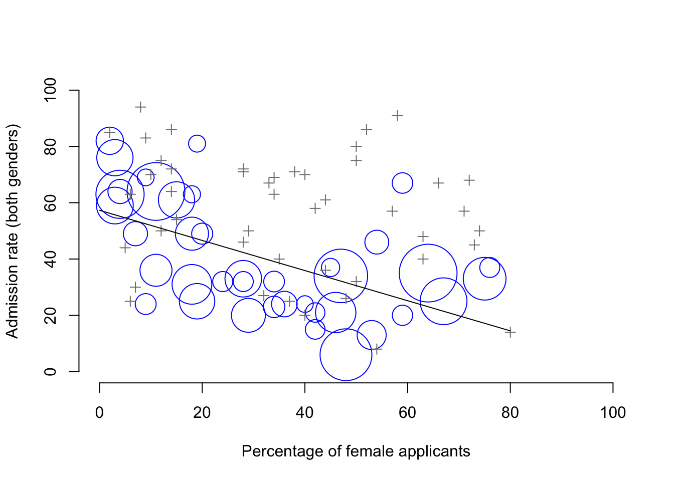
Figure 1.1: The Berkeley 1973 college admissions data. This figure plots the admission rate for the 85 departments that had at least one female applicant, as a function of the percentage of applicants that were female. The plot is a redrawing of Figure 1 from Bickel, Hammel, and O’Connell (1975). Circles plot departments with more than 40 applicants; the area of the circle is proportional to the total number of applicants. The crosses plot department with fewer than 40 applicants.
Before leaving this topic entirely, I want to point out something else really critical that is often overlooked in a research methods class. Statistics only solves part of the problem. Remember that we started all this with the concern that Berkeley’s admissions processes might be unfairly biased against female applicants. When we looked at the “aggregated” data, it did seem like the university was discriminating against women, but when we “disaggregate” and looked at the individual behaviour of all the departments, it turned out that the actual departments were, if anything, slightly biased in favour of women. The gender bias in total admissions was caused by the fact that women tended to self-select for harder departments. From a legal perspective, that would probably put the university in the clear. Postgraduate admissions are determined at the level of the individual department (and there are good reasons to do that), and at the level of individual departments, the decisions are more or less unbiased (the weak bias in favour of females at that level is small, and not consistent across departments). Since the university can’t dictate which departments people choose to apply to, and the decision making takes place at the level of the department it can hardly be held accountable for any biases that those choices produce.
That was the basis for my somewhat glib remarks earlier, but that’s not exactly the whole story, is it? After all, if we’re interested in this from a more sociological and psychological perspective, we might want to ask why there are such strong gender differences in applications. Why do males tend to apply to engineering more often than females, and why is this reversed for the English department? And why is it it the case that the departments that tend to have a female-application bias tend to have lower overall admission rates than those departments that have a male-application bias? Might this not still reflect a gender bias, even though every single department is itself unbiased? It might. Suppose, hypothetically, that males preferred to apply to “hard sciences” and females prefer “humanities.” And suppose further that the reason for why the humanities departments have low admission rates is because the government doesn’t want to fund the humanities (Ph.D. places, for instance, are often tied to government funded research projects). Does that constitute a gender bias? Or just an unenlightened view of the value of the humanities? What if someone at a high level in the government cut the humanities funds because they felt that the humanities are “useless chick stuff.” That seems pretty blatantly gender biased. None of this falls within the purview of statistics, but it matters to the research project. If you’re interested in the overall structural effects of subtle gender biases, then you probably want to look at both the aggregated and disaggregated data. If you’re interested in the decision making process at Berkeley itself then you’re probably only interested in the disaggregated data.
In short there are a lot of critical questions that you can’t answer with statistics, but the answers to those questions will have a huge impact on how you analyse and interpret data. And this is the reason why you should always think of statistics as a tool to help you learn about your data, no more and no less. It’s a powerful tool to that end, but there’s no substitute for careful thought.
1.6 A brief introduction to research design
To consult the statistician after an experiment is finished is often merely to ask him to conduct a post mortem examination. He can perhaps say what the experiment died of.
– Sir Ronald Fisher2
Note that this section is “special” in two ways. Firstly, it’s much more psychology-specific than the later chapters. Secondly, it focuses much more heavily on the scientific problem of research methodology, and much less on the statistical problem of data analysis. Nevertheless, the two problems are related to one another, so it’s traditional for stats textbooks to discuss the problem in a little detail. This chapter relies heavily on Campbell and Stanley (1963) for the discussion of study design, and Stevens (1946) for the discussion of scales of measurement. Later versions will attempt to be more precise in the citations.
1.6.1 Some thoughts about psychological measurement
Measurement itself is a subtle concept, but basically it comes down to finding some way of assigning numbers, or labels, or some other kind of well-defined descriptions to “stuff.” So, any of the following would count as a psychological measurement:
- My age is 33 years.
- I do not like anchovies.
- My chromosomal gender is male.
- My self-identified gender is male.3
In the short list above, the bolded part is “the thing to be measured,” and the italicised part is “the measurement itself.” In fact, we can expand on this a little bit, by thinking about the set of possible measurements that could have arisen in each case:
- My age (in years) could have been 0, 1, 2, 3 …, etc. The upper bound on what my age could possibly be is a bit fuzzy, but in practice you’d be safe in saying that the largest possible age is 150, since no human has ever lived that long.
- When asked if I like anchovies, I might have said that I do, or I do not, or I have no opinion, or I sometimes do.
- My chromosomal gender is almost certainly going to be male (XY) or female (XX), but there are a few other possibilities. I could also have Klinfelter’s syndrome (XXY), which is more similar to male than to female. And I imagine there are other possibilities too.
- My self-identified gender is also very likely to be male or female, but it doesn’t have to agree with my chromosomal gender. I may also choose to identify with neither, or to explicitly call myself transgender.
As you can see, for some things (like age) it seems fairly obvious what the set of possible measurements should be, whereas for other things it gets a bit tricky. But I want to point out that even in the case of someone’s age, it’s much more subtle than this. For instance, in the example above, I assumed that it was okay to measure age in years. But if you’re a developmental psychologist, that’s way too crude, and so you often measure age in years and months (if a child is 2 years and 11 months, this is usually written as “2;11”). If you’re interested in newborns, you might want to measure age in days since birth, maybe even hours since birth. In other words, the way in which you specify the allowable measurement values is important.
Looking at this a bit more closely, you might also realise that the concept of “age” isn’t actually all that precise. In general, when we say “age” we implicitly mean “the length of time since birth.” But that’s not always the right way to do it. Suppose you’re interested in how newborn babies control their eye movements. If you’re interested in kids that young, you might also start to worry that “birth” is not the only meaningful point in time to care about. If Baby Alice is born 3 weeks premature and Baby Bianca is born 1 week late, would it really make sense to say that they are the “same age” if we encountered them “2 hours after birth?” In one sense, yes: by social convention, we use birth as our reference point for talking about age in everyday life, since it defines the amount of time the person has been operating as an independent entity in the world, but from a scientific perspective that’s not the only thing we care about. When we think about the biology of human beings, it’s often useful to think of ourselves as organisms that have been growing and maturing since conception, and from that perspective Alice and Bianca aren’t the same age at all. So you might want to define the concept of “age” in two different ways: the length of time since conception, and the length of time since birth. When dealing with adults, it won’t make much difference, but when dealing with newborns it might.
Moving beyond these issues, there’s the question of methodology. What specific “measurement method” are you going to use to find out someone’s age? As before, there are lots of different possibilities:
- You could just ask people “how old are you?” The method of self-report is fast, cheap and easy, but it only works with people old enough to understand the question, and some people lie about their age.
- You could ask an authority (e.g., a parent) “how old is your child?” This method is fast, and when dealing with kids it’s not all that hard since the parent is almost always around. It doesn’t work as well if you want to know “age since conception,” since a lot of parents can’t say for sure when conception took place. For that, you might need a different authority (e.g., an obstetrician).
- You could look up official records, like birth certificates. This is time consuming and annoying, but it has its uses (e.g., if the person is now dead).
1.6.2 Operationalisation: defining your measurement
All of the ideas discussed in the previous section all relate to the concept of operationalisation. To be a bit more precise about the idea, operationalisation is the process by which we take a meaningful but somewhat vague concept, and turn it into a precise measurement. The process of operationalisation can involve several different things:
- Being precise about what you are trying to measure. For instance, does “age” mean “time since birth” or “time since conception” in the context of your research?
- Determining what method you will use to measure it. Will you use self-report to measure age, ask a parent, or look up an official record? If you’re using self-report, how will you phrase the question?
- Defining the set of the allowable values that the measurement can take. Note that these values don’t always have to be numerical, though they often are. When measuring age, the values are numerical, but we still need to think carefully about what numbers are allowed. Do we want age in years, years and months, days, hours? Etc. For other types of measurements (e.g., gender), the values aren’t numerical. But, just as before, we need to think about what values are allowed. If we’re asking people to self-report their gender, what options to we allow them to choose between? Is it enough to allow only “male” or “female?” Do you need an “other” option? Or should we not give people any specific options, and let them answer in their own words? And if you open up the set of possible values to include all verbal response, how will you interpret their answers?
Operationalisation is a tricky business, and there’s no “one, true way” to do it. The way in which you choose to operationalise the informal concept of “age” or “gender” into a formal measurement depends on what you need to use the measurement for. Often you’ll find that the community of scientists who work in your area have some fairly well-established ideas for how to go about it. In other words, operationalisation needs to be thought through on a case by case basis. Nevertheless, while there a lot of issues that are specific to each individual research project, there are some aspects to it that are pretty general.
Before moving on, I want to take a moment to clear up our terminology, and in the process introduce one more term. Here are four different things that are closely related to each other:
- A theoretical construct. This is the thing that you’re trying to take a measurement of, like “age,” “gender” or an “opinion.” A theoretical construct can’t be directly observed, and often they’re actually a bit vague.
- A measure. The measure refers to the method or the tool that you use to make your observations. A question in a survey, a behavioural observation or a brain scan could all count as a measure.
- An operationalisation. The term “operationalisation” refers to the logical connection between the measure and the theoretical construct, or to the process by which we try to derive a measure from a theoretical construct.
- A variable. Finally, a new term. A variable is what we end up with when we apply our measure to something in the world. That is, variables are the actual “data” that we end up with in our data sets.
In practice, even scientists tend to blur the distinction between these things, but it’s very helpful to try to understand the differences.
1.6.3 The “role” of variables: predictors and outcomes
Okay, I’ve got one last piece of terminology that I need to explain to you before moving away from variables. Normally, when we do some research we end up with lots of different variables. Then, when we analyse our data we usually try to explain some of the variables in terms of some of the other variables. It’s important to keep the two roles “thing doing the explaining” and “thing being explained” distinct. So let’s be clear about this now. Firstly, we might as well get used to the idea of using mathematical symbols to describe variables, since it’s going to happen over and over again. Let’s denote the “to be explained” variable \(Y\), and denote the variables “doing the explaining” as \(X_1\), \(X_2\), etc.
Now, when we doing an analysis, we have different names for \(X\) and \(Y\), since they play different roles in the analysis. The classical names for these roles are independent variable (IV) and dependent variable (DV). The IV is the variable that you use to do the explaining (i.e., \(X\)) and the DV is the variable being explained (i.e., \(Y\)). The logic behind these names goes like this: if there really is a relationship between \(X\) and \(Y\) then we can say that \(Y\) depends on \(X\), and if we have designed our study “properly” then \(X\) isn’t dependent on anything else. However, I personally find those names horrible: they’re hard to remember and they’re highly misleading, because (a) the IV is never actually “independent of everything else” and (b) if there’s no relationship, then the DV doesn’t actually depend on the IV. And in fact, because I’m not the only person who thinks that IV and DV are just awful names, there are a number of alternatives that I find more appealing. The terms that I’ll use in these notes are predictors and outcomes. The idea here is that what you’re trying to do is use \(X\) (the predictors) to make guesses about \(Y\) (the outcomes).4 This is summarised in Table 1.2.
| role of the variable | classical name | modern name |
|---|---|---|
| to be explained | dependent variable (DV) | outcome |
| to do the explaining | independent variable (IV) | predictor |
1.6.4 Experimental and non-experimental research
Video: Experimental, Quasi-, and Non-Experimental Research Designs
One of the big distinctions that you should be aware of is the distinction between “experimental research” and “non-experimental research.” When we make this distinction, what we’re really talking about is the degree of control that the researcher exercises over the people and events in the study.
1.6.4.1 Experimental research
The key features of experimental research is that the researcher controls all aspects of the study, especially what participants experience during the study. In particular, the researcher manipulates or varies the predictor variables (IVs), and then allows the outcome variable (DV) to vary naturally. The idea here is to deliberately vary the predictors (IVs) to see if they have any causal effects on the outcomes. Moreover, in order to ensure that there’s no chance that something other than the predictor variables is causing the outcomes, everything else is kept constant or is in some other way “balanced” to ensure that they have no effect on the results. In practice, it’s almost impossible to think of everything else that might have an influence on the outcome of an experiment, much less keep it constant. The standard solution to this is randomisation: that is, we randomly assign people to different groups, and then give each group a different treatment (i.e., assign them different values of the predictor variables). We’ll talk more about randomisation later in this course, but for now, it’s enough to say that what randomisation does is minimise (but not eliminate) the chances that there are any systematic difference between groups.
Let’s consider a very simple, completely unrealistic and grossly unethical example. Suppose you wanted to find out if smoking causes lung cancer. One way to do this would be to find people who smoke and people who don’t smoke, and look to see if smokers have a higher rate of lung cancer. This is not a proper experiment, since the researcher doesn’t have a lot of control over who is and isn’t a smoker. And this really matters: for instance, it might be that people who choose to smoke cigarettes also tend to have poor diets, or maybe they tend to work in asbestos mines, or whatever. The point here is that the groups (smokers and non-smokers) actually differ on lots of things, not just smoking. So it might be that the higher incidence of lung cancer among smokers is caused by something else, not by smoking per se. In technical terms, these other things (e.g. diet) are called “confounds,” and we’ll talk about those in just a moment.
In the meantime, let’s now consider what a proper experiment might look like. Recall that our concern was that smokers and non-smokers might differ in lots of ways. The solution, as long as you have no ethics, is to control who smokes and who doesn’t. Specifically, if we randomly divide participants into two groups, and force half of them to become smokers, then it’s very unlikely that the groups will differ in any respect other than the fact that half of them smoke. That way, if our smoking group gets cancer at a higher rate than the non-smoking group, then we can feel pretty confident that (a) smoking does cause cancer and (b) we’re murderers.
1.7 Causality, Research, and Statistics
Text by David Schuster
1.7.1 Experimental, Quasi-Experimental, and Non-Experimental Studies
In this section, I would like to add a bit more precision to the general concepts explained by Navarro (2018).
Research psychology is a process of identifying constructs and describing how they relate to other constructs. We can classify research designs as experiments, quasi-experiments, and non-experiments.
Experiments are the only kind of research that shows causal relationships (that is, that construct A causes a change in construct B). So an experiment could show if smoking causes lung cancer. To do this, experiments need two things (or they are not experiments)
All experiments have a manipulation. This means that the experimenter changes something within the environment of the experiment (called an independent variable) to see if it causes a change in the outcome (called a dependent variable). For our smoking example, a manipulation would be assigning one group of participants to a lifetime of smoking and another group of participants to a lifetime of no smoking.
Experiments require random assignment. The experimenter decides when to vary the levels of the manipulation (change the manipulation) based on random assignment. Random assignment means that every participant has the same chance as being in one condition as another. For our smoking example, random assignment means each participant has a 50% chance of being in the smoking group.
As may be clear from the smoking example, we cannot always do experiments because of ethical (it would be wrong to assign people to smoke) or practical reasons (you cannot randomly assign people to genders, for example). The solution is a quasi- or non-experimental study.
In summary: experiments are powerful because they uniquely demonstrate causality (causal relationships). However, experiments require a manipulation and random assignment, which are not always possible.
In a quasi-experimental study, there is a manipulation but no random assignment. Whenever participants are assigned to levels of a manipulation non-randomly, the research is quasi-experimental. In a quasi-experimental smoking study, we could ask people if they had smoked before and assign them to smoking or non-smoking groups based on that answer.
In summary: quasi-experiments do not require random assignment, but they do not show casual relationships.
In a non-experimental study, no manipulation is done. If you want to look at the effects of gender on lung cancer, you would simply observe (collect data on) the genders of patients. By only observing, you would not be manipulating gender.
The differences between quasi- and non-experimental studies are sometimes slight (Pedhauzer & Schmelkin, 1991); if the researcher is manipulating an IV, then the work is quasi-experimental.
In summary: non-experimental studies are observational. Like quasi-experimental studies, they do not show causal relationships.
It’s worth repeating that only experiments demonstrate causality. Quasi- and non-experiments can show that a relationship exists but do not say whether one variable causes the other. Any non-causal relationship has three possible explanations:
- A \(\rightarrow\) B one variable causes another; in an experiment, this is the only explanation
- B \(\leftarrow\) A the relationship is reversed; the first variable is actually the outcome
- C \(\rightarrow\) A; C \(\rightarrow\) B a third variable exists that was not measured in the study; the third variable causes a change in both A and B. There are many ‘C’ variables, potentially.
In a non-experimental smoking study, you could not say whether smoking causes lung cancer or people who are predisposed to lung cancer are more likely to smoke. A third possibility is that a separate, third variable causes both lung cancer and a desire to smoke.
1.7.2 Demonstrating Causality
In the 19th century, John Stewart Mill said that we could be satisfied that a relationship is causal if the following three things could be demonstrated:
- The cause preceded the effect
- The cause was related to the effect
- We can find no plausible alternative explanation for the effect other than the cause
Experiments aim to identify causal relationships by manipulating something, observing the outcome, seeing a relationship, and using various methods to reduce other explanations.
1.7.3 Statistics and Causality
Statistics are an important tool for establishing causality, but it’s important to know that the choice of statistical technique does not affect the level of causal evidence; demonstrating causality is the job of the research design, not the statistics.
A common misconception arises from the term correlational research design, which people use as a label for quasi-experimental and non-experimental research. It is easy to confuse this term with correlation which is a statistical technique.
Recall that statistics has two branches: Descriptive stats provides tools to summarize variability. Inferential stats provides tools for generalizing samples to populations.
To demonstrate causality, we need to satisfy Mill’s second requirement. Inferential statistics can help us do that. Two techniques are particularly useful: correlation (and its statistic r) and the t¬-test (and its statistic, t). Next, we will see how these techniques work.
1.7.4 Validity and Reliability
Text by David Schuster
1.7.4.1 Define validity and reliability
Reliability and validity are fundamental to critiquing psychological research and to developing your own high-quality research. There are different types of validity and reliability that are relevant to us, which sometimes confuses people. Because of this, introductory textbooks often present convoluted definitions of these concepts. Fortunately, the real definitions are simple:
Reliability means consistency. Something is reliable if it is consistent. The more consistency, the more reliability.
Validity means truth. Something is valid if it is true. Truth is either-or; there is no such thing as “more true” or “less true.”
In other words, good psychological science requires certain types of consistency and for some of the claims we make to be true. Next, we will look at the specific kinds of reliability and validity that are important for scientists.
1.7.4.2 Types of consistency = Types of Reliability
Here are arguably the three most important types of reliability:
| Type of Reliability | Situation | Definition | How to assess |
|---|---|---|---|
| Test-retest | You administer a measure to a participant, then wait some period of time, and give them the test again. The participant’s true score on the measure has not changed (e.g., IQ, personality). | The extent to which a measure is consistent across different administrations | Look for a correlation between the two administrations |
| Interrater | A measure involves two or more raters who record subjective observations (e.g., counting the number of times a participant has a tic, counting the number of times a married couple shows affection) | The extent to which two observers are consistent in their ratings | Look for a correlation between the two raters |
| Internal consistency | You are measuring a construct using several items (e.g., five items all rating your enjoyment of a course) | The extent to which items on a measure are consistent with each other; expected if the items measure the same construct | Cronbach’s alpha (.7 is acceptable, .8 is good, and .9 is excellent) |
1.7.4.3 Validity is a property of inferences
Validity is a specific kind of truth. Validity is the truth of an inference, or a claim. In other words, validity is a property of inferences. An inference (a claim) is valid if it is true.
For example, I could claim that the earth is round. Hopefully, it is a claim that you accept as being true. If you agree, then you could label my claim as valid.
Validity in research is frequently misunderstood, which leads to bizarre and confusing definitions of validity. There is no such thing as “a valid study.” Only claims about the study are valid or not. There is also no such thing as “a valid researcher.” A researcher can make claims. Only the researcher’s claims are valid or not. There is also no such thing as “more valid” or “increasing validity.” Validity is truth of a claim. Either a claim is true, or it is not.
For better or for worse, we usually don’t know with 100% certainty if a claim is true or false (if we did, we wouldn’t need the research). Therefore, research methods get very interesting when we listen to other researcher’s claims and then debate if we agree with them or not. When we do this, we are evaluating the validity of claims made about the study. Next, let’s look at different types of claims (inferences) that are made in research.
1.7.4.4 Types of inferences in a study = Types of validity
Here are some of the most important types of validity.
| Type of Validity | Type of Claim | Definition | Example claim |
|---|---|---|---|
| Construct validity | The study operations represent the constructs of interest | The truth of claims that study operations match study constructs | “The Stanford-Binet was used to measure IQ” |
| Internal validity | The study IV caused a change in the study DV | The truth of claims that the IV causes changes in the DV | “The control group reported lower levels of stress than the experimental group, suggesting that the manipulation raised stress.” |
| External validity | The study results apply to situation X | The truth of claims that the findings will apply as participants/units/variables/settings change. | “Although data were collected from college students, a similar effect would be expected in working adults.” |
| Statistical conclusion validity | The statistical analysis was significant or not significant | The truth of claims about the size and direction of the relationship between the IV and the DV. Or, that the statistical results are correct. | “p < .05, indicating a significant difference” |
Finally, you might encounter these other types of validity, but they are less clearly defined and evaluated:
- Content validity: The truth of claims that a measure adequately samples (includes the important elements of) the domain of interest. For example, if IQ includes both verbal and math ability, an IQ test would need to have both verbal and math items.
- Face validity: The truth of claims that a study operation “seems like” the construct. For example, a study about distractions from mobile devices might not support claims of “seeming real” if the phone in the study is a paper mockup.
- Criterion validity: The truth of claims that a measure can predict or correlate with some outcome of interest. A personality test as part of a job application would have criterion validity if it predicted applicants’ success in the job.
1.7.4.5 Threats to validity
Threats to validity are specific reasons why an inference about a study is wrong. They can help us anticipate problems in the design of our own research. The best way to address threats to validity is to change the design of our research. Understanding threats to validity also helps you critique research done by others.
References
Earlier versions of these notes incorrectly suggested that they actually were sued – apparently that’s not true. There’s a nice commentary on this here: https://www.refsmmat.com/posts/2016-05-08-simpsons-paradox-berkeley.html. A big thank you to Wilfried Van Hirtum for pointing this out to me!↩︎
Presidential Address to the First Indian Statistical Congress, 1938. Source: http://en.wikiquote.org/wiki/Ronald_Fisher↩︎
Well… now this is awkward, isn’t it? This section is one of the oldest parts of the book, and it’s outdated in a rather embarrassing way. I wrote this in 2010, at which point all of those facts were true. Revisiting this in 2018… well I’m not 33 any more, but that’s not surprising I suppose. I can’t imagine my chromosomes have changed, so I’m going to guess my karyotype was then and is now XY. The self-identified gender, on the other hand… ah. I suppose the fact that the title page now refers to me as Danielle rather than Daniel might possibly be a giveaway, but I don’t typically identify as “male” on a gender questionnaire these days, and I prefer “she/her” pronouns as a default (it’s a long story)! I did think a little about how I was going to handle this in the book, actually. The book has a somewhat distinct authorial voice to it, and I feel like it would be a rather different work if I went back and wrote everything as Danielle and updated all the pronouns in the work. Besides, it would be a lot of work, so I’ve left my name as “Dan” throughout the book, and in ant case “Dan” is a perfectly good nickname for “Danielle,” don’t you think? In any case, it’s not a big deal. I only wanted to mention it to make life a little easier for readers who aren’t sure how to refer to me. I still don’t like anchovies though :-)↩︎
Annoyingly, though, there’s a lot of different names used out there. I won’t list all of them – there would be no point in doing that – other than to note that R often uses “response variable” where I’ve used “outcome,” and a traditionalist would use “dependent variable.” Sigh. This sort of terminological confusion is very common, I’m afraid.↩︎